Salient Search

(1)

University of Windsor University of Windsor

Scholarship at UWindsor

Electronic Theses and Dissertations Theses, Dissertations, and Major Papers

2011

Salient Search

Jonathan Vermette University of Windsor

Follow this and additional works at: https://scholar.uwindsor.ca/etd

Recommended Citation Recommended Citation

Vermette, Jonathan, "Salient Search" (2011). Electronic Theses and Dissertations. 342.

https://scholar.uwindsor.ca/etd/342

(2)

SALIENT SEARCH

by

JONATHAN VERMETTE

A Thesis

Submitted to the Faculty of Graduate Studies through Computer Science

in Partial Fulfilment of the Requirements for the Degree of Master of Science at the

University of Windsor

(3)

SALIENT SEARCH by

JONATHAN VERMETTE

APPROVED BY:

Dr. Phil Graniero

Department of Earth and Environmental Sciences

Dr. Dan Wu

School of Computer Science

Dr. Scott Goodwin School of Computer Science

Dr. Subir Bandyopadhyay Chair of Defense School of Computer Science

(4)

Author’s Declaration of Originality

I hereby certify that I am the sole author of this thesis and that no part of this thesis has been published or submitted for publication.

I certify that, to the best of my knowledge, my thesis does not infringe upon anyone’s copyright nor violate any proprietary rights and that any ideas, techniques, quotations, or any other material from the work of other people included in my thesis, published or otherwise, are fully acknowledged in accordance with the standard referencing practices. Furthermore, to the extent that I have included copyrighted material that surpasses the bounds of fair dealing within the meaning of the Canada Copyright Act, I certify that I have obtained a written permission from the copyright owner(s) to include such material(s) in my thesis and have included copies of such copyright clearances to my appendix.

(5)

Abstract

All real-time pathfinding algorithms suffer from some degree of suboptimal behaviour on the part of the agent. A consequence of the need to perform a move before it is guaranteed to be optimal, this is inversely proportional to the amount of effort given to planning between each move.

Many real-time algorithms employ a constant-bounded local search to plan a single move at a time. However they need multiple trials to converge on an optimal solution. More recent hierarchical approaches produce good results after a single trial, but rely on extensive pre-processing, limiting their use in dynamic environments. A newer algorithm, Time Bounded A*, conducts a global A* to find an optimal path on the first trial, while creating partial paths for an agent to follow. However, harder search problems can induce the appearance of indecisiveness on the part of the agent as all of its time is spent moving back and forth between subgoals.

(6)

Dedication

(7)

Acknowledgements

I would first like to thank my supervisor, Dr. Scott Goodwin for inviting me to work in Game AI, and providing plenty of guidance and direction during my time as a graduate student. He has helped me win an argument that has gone on between parents and kids all over: All those years playing video games, instead of being a waste of my time have put me on the path to a satisfying and challenging career.

I would like to the thank the members of the thesis committee for taking time out of their schedules to review this thesis, and for providing valuable feedback during the proposal. Their suggestions guided this work.

Special thanks goes to Dr. Nathan Sturtevant, previously of the University of Alberta, for replying to my early enquiries into his work and for providing access to the code repository for his Hierarchical Open Graph project. The dataset of maps used in this thesis were derived from the set provided through this framework.

Finally, I would like to thank the Montana’s restaurant of Windsor, Ontario for providing table coverings that patrons are encouraged to draw on. It was here while having lunch one afternoon that Dr. Goodwin and I sketched out the initial idea that became Salient Search. And sketch is the key word. From this meeting I suspect that this thesis has the curious distinction of being among the first to be conceived in crayon and butcher’s paper.

(8)

List of Tables

4.1 NS Values . . . 43

4.2 Travel Ratio of TBA* . . . 48

4.3 Travel Ratio of Salient Search . . . 48

4.4 Mean Backwards Steps for Agents in SS, TBA* . . . 53

4.5 ANOVA For Backwards Steps . . . 53

4.6 Mean Changes in Direction of Travel for SS, TBA* . . . 56

4.7 ANOVA For Changes in Direction . . . 56

4.8 Mean Backwards Steps for Agents in SS, TBA* On Harder Maps . . 61

4.9 ANOVA For Backwards Steps On Harder Maps . . . 61

4.10 Mean Changes in Direction of Travel For SS, TBA* On Harder Maps 62 4.11 ANOVA For Changes In Direction of Travel On Harder Maps . . . . 63

A.1 Heuristic Error Breakdown By Map . . . 75

A.2 Travel Ratio of Salient Search on Cardinal Grid-Type . . . 75

(12)

List of Figures

1.1 Types of Problem Domains . . . 2

2.1 A* In Action. . . 6

2.2 A Heuristic Depression for LRTA* . . . 9

2.3 An Example of Graph Abstraction . . . 13

2.4 PR LRTA* . . . 15

2.5 Illustration of Successive Subgoals of TBA* . . . 19

2.6 Agent Backtracking in TBA* . . . 20

3.1 Successive Paths With No Common Section. . . 24

3.2 An Agent Moving Towards Subgoalg . . . 25

3.3 Visual Representation of a Salient . . . 26

3.4 The Salient on a Search Tree . . . 29

3.5 The Salient List . . . 32

4.1 An Example Map . . . 39

4.2 Grid Types . . . 39

4.3 Illustration of Corner Cutting . . . 40

4.4 Histrogram of A* Costs For Different Map Styles . . . 44

4.5 Scatterplot of Heuristic Error. . . 46

4.6 Travel Ratio of Salient Search With AD Strategy . . . 49

(13)

4.8 Two Different Behaviours From Travel Paths. . . 52

4.9 A Forking Path. . . 55

4.10 Backtracking Behaviours . . . 57

4.11 Four Maps With Harder Searches . . . 58

(14)

List of Algorithms

1 A* . . . 5

2 Learning Real-Time A* (LRTA*) . . . 8

3 Priortized LRTA* (P-LRTA*) . . . 12

4 Time Bounded A* (TBA*) . . . 17

5 Salient Search . . . 30

6 SalientA∗₍_{lists, start, goal, N} E, NS) . . . 31

7 Salient Search: expandNext . . . 31

(15)

Glossary

A*

An informed search algorithm. A best-first algorithm, notable for being opti-mally efficient; A* expands the fewest number of nodes while guaranteeing the path found is optimal.

backtracking

A move made by an agent in real-time pathfinding to return to a previously visited node, in pursuit of a new subgoal.

closed list

A data structure used in pathfinding algorithms to identify search nodes that have already been expanded.

heuristic

A function to estimate the optimal distance between two nodes or states in a problem space. Heuristic functions that never overestimate the optimal distance are said to be admissible, and important property.

heuristic error

The difference between a heuristic estimate and the true optimal cost between two nodes or states in a problem space.

learning real-time search

(16)

to their ‘true’ value. LRTA* is a notable example.

most promising node

The next node to be expanded in best-first search. In A*, the most promising node is the node on the open list with the lowest f-score. In TBA*, the most promising node at different points in time form the endpoints of the various paths created.

octile grid

A two-dimensional grid space where diagonal moves are permitted.

optimal path

Between two points, the optimal path is that which has the lowest cost to traverse.

open list

A data structure used in pathfinding algorithms to identify search nodes that are ready to be expanded.

pathfinding

The problem of identifying a series of moves or transformations in a problem space that produces a desired state or solution.

real-time pathfinding

Any pathfinding algorithm that incorporates both planning and execution by an agent, while guaranteeing a constant bound on the amount of planning for every execution, independent of the size of the problem space.

resource limit

A limit defining the bound on planning in a real-time algorithm.

(17)

salient expansion

Node expansion conducted on nodes defined by the salient list.

salient list

The data structure that describes which nodes on the open list are part of the salient.

salient search

A real-time pathfinding algorithm derived from TBA*.

salient root

The node that initially describes a salient. When expanded, all successor nodes are referenced by the salient list.

strategy

A decision function to choose between the best nodes of the open and salient lists.

subgoal

Some intermediate destination node that the agent is moving towards, and not necessarily the stated goal of the problem

suboptimality

The ratio to which a path between two points is greater in cost than the optimal.

time bounded A*

A real-time pathfinding algorithm. Notable for employing a global search tech-nique while ensuring a constant bound on planning.

travel ratio

(18)

Chapter 1 Introduction

1.1 Problem Domain

This is a thesis on pathfinding. Broadly speaking, pathfinding is the problem of determining a series of moves or transformations (thepath) that results in a solution state. Examples include moving through an environment in a computer game to some desired destination, a series of commands to manipulate a robotic arm to a given configuration, or the fewest moves to a checkmate of an opponent in chess. Pathfinding algorithms can be applied to any problem that can be expressed in terms of a weighted, directed graph where each possible state of a problem is expressed in terms of a node. In general, a pathfinding problem can be expressed by the tuple

{P,_S,_G,_E, h_}, where:

• P is theproblem space ordomain. The complete set of possible states, or nodes, of the problem.

• S is the initial or start state or node.

• G is the goal node(s).

(19)

Figure 1.1: Game trees and Virtual Spaces, two types of problem domains where pathfinding applies.

• h is a heuristic function.

Two examples of problem domains are illustrated in Figure 1.1. On the left is a portion of a game tree for Tic-Tac-Toe. From the initial empty board at the beginning of the game, a series of moves are possible alternating the placement of X’s and O’s on the board, creating successive configurations. Each possible configuration of X’s and O’s comprises a single state in this game tree. A goal state would be any state with three X’s or 3 O’s in a row, depending on which is desired. If the symmetrical configurations† _{are collapsed into a single state, then the game tree for Tic-Tac-Toe}

is actually quite small [Dew89]. Other examples of games that are readily described by game trees include Chess, Checkers, Go, or puzzles like the 8-puzzle or a Rubik’s Cube.

On the right is an example of a virtual space: a grid-based map taken from a computer game [CSE00] that is used later in this thesis. In a virtual space such as this, states are each (x, y) coordinate cell, and edges defined for each move between adjacent cells.

This thesis works in a subset of pathfinding, known as real-time pathfinding. Real-time pathfinding algorithms incorporate an agent performing transformations

†_{For example, the topmost state represents four different legal moves in the game, if one rotates}

(20)

alongside the search for a solution. Also, by the definition in [BSLY07], a real-time

pathfinding algorithm is one that can perform a constant amount of work between a given time interval, regardless of the size of the problem space. More detail on the definition is in [Koe01].

[BSLY07] notes that the real-time pathfinding algorithms remain important in robotics (citing [KS98, Koe98, KTN+

99, KTS03]) and video games. Robotics systems are known to use variants of the D* algorithm [Ste94], including D*-Lite and AD* [KL02, LFG+

05, FHL08], especially autonomous vehicle navigation.

1.2 Contribution of this Thesis

In this thesis we introduce a variant of real-time heuristic search dubbed Salient Search. This algorithm builds on the Time Bounded A* (TBA*) algorithm [BBS09]. Salient Search allows for targeted expansions of a chosen subset of the open list through the use of a secondary data structure, while preserving the constant time guarantees that define real-time pathfinding. Also used is a secondary function called a strategy to influence intermediate goal selection and weighting of the open list. In addition to describing Salient Search, this thesis provides the results of an empirical analysis of Salient Search versus TBA*.

All real-time pathfinding algorithms suffer from some degree of suboptimal be-haviour on the part of the agent. A consequence of the need to perform a move before it is guaranteed to be optimal, this is inversely proportional to the amount of effort given to planning between each move. In certain applications like large scale crowd simulation or real-time strategy computer games, computing time devoted to pathfinding must be further divided up amongst many agents, each with their own separate search problems. As a result, the limited computational budget magnifies the scale of this suboptimal behaviour.

(21)

difficult search and/or small planning windows, the paths can be wildly divergent, sharing no common portion beyond their starting location. In this circumstance, an agent would make little progress before requiring a return to the starting location to continue forward. This indecisiveness or ‘squirreliness’ on the part of the agent is undesirable in the context of computer games. A user witnessing such behaviour may issue an additional search command thinking something is wrong, effectively throwing away any progress made as search begins anew.

The algorithm proposed in this thesis, Salient Search, performs better than TBA* in avoiding this behaviour for small planning windows. The experiments presented in Chapter 4 show that the features introduced in Salient Search cause an agent to change direction fewer times than they would using TBA*. Further, the effect is stronger with more difficult problems.

1.3 Organization of this Thesis

The rest of this thesis is organised as follows: in Chapter 2 a brief overview of real-time pathfinding is provided. Several milestone techniques in the field are described, showing the evolution of real-time pathfinding. An in-depth look at TBA* finishes the review of past techniques. TBA* is a recent algorithm from which Salient Search is derived. Chapter 3 introduces the Salient Search algorithm itself, which forms the main contribution of this thesis. The two distinguishing features of the algorithm are the Salient List and Salient Strategy. Chapter 4 presents an empirical study of Salient Search. This study compares the behaviour of Salient Search against its parent algorithm, TBA*. Chapter 5 provides some concluding remarks, as well as observations on possible future work with Salient Search.

(22)

Chapter 2 Real-time Pathfinding

2.1 A*

The most widely known best-first search algorithm is the A* algorithm, introduced by Hart in [HNR68].

Algorithm 1 A*

1: add Start to OPEN

2: goalF ound_←f alse

3: while OPEN6= empty AND Goal not found do

4: next_← OPEN with lowest f

5: neighbours _←expand next

6: add next to CLOSED

7: for all neighbour in neighbours do

8: if CLOSED contains neighbour then

9: continue

10: else if OPEN containsneighbour then

11: update neighbour

12: else

13: add neighbour to OPEN

14: end if

15: end for

16: end while

(23)

expanded - its neighbors have theirf-scores calculated and are placed onto the open list (lines 7-15).

The next node from the open list is the one with the best (e.g. lowest) f-score, and similarly processed (lines 4-6). This process is repeated until either the goal is reached or the open list is first exhausted (line 3).

When the goal is found to be reachable from the start, a path is traced backwards from the goal. This is accomplished by having each node maintaining a parent refer-ence to the node that produced it. In this way the open and closed lists form a tree data structure, with the open list forming the leaf nodes, and the starting location as the root. S G 000 000 000 111 111 111 00 00 11 11 00 00 00 11 11 11 00 00 00 11 11 11 00 00 11 11 000 000 111 111 00 00 11 11 00 00 11 11 00 00 00 11 11 11 00 00 00 11 11 11 000 000 000 111 111 111 000 000 111 111 000 000 111 111 000 000 000 111 111 111 00 00 00 11 11 11 000 000 111 111 000 000 000 111 111 111 00 00 11 11 000 000 111 111 00 00 00 11 11 11 00 00 00 11 11 11 00 00 11 11 00 00 00 11 11 11 S G

Figure 2.1: A snapshot of A* in action finding a solution from S to G. A* uses the open list to process or ‘expand’ nodes in a best-first fashion, adding to or updating neighbouring nodes on the open list where necessary. Processed nodes are put onto the closed list. Here, closed list nodes are shaded gray, surrounded by open list nodes (the hatched nodes) to be processed.

Calculating f(n)

As mentioned, determining the ordering of expansion is determined by calculating a score for each node n. In A* this equation takes the form of f(n):

(24)

g(n) is thetraversal cost, exactly how much it costs to transition tonfrom the starting state by adding up all costs in between. This is determined by g(n) for the parent state plus the transition cost to this state from the parent state. For the starting nodeg(n) = 0.

h(n) is the heuristic function. This function is an informed ‘guess’ as to how much it will cost to transition to the goal state fromn. In other words, an estimate of

g(goal)₋g(n). Heuristics are usually described in terms of the transition costs. For example, for a Rubik’s cube where each state describes a configuration of the faces, the cost and transitions can be the number of and type of planar rotations of the toy. A (not efficient) example of a heuristic for a Rubik’s cube would be a count of the number of faces solved; positioned and oriented as they would be in the finished cube. In a computer game, it may be the Euclidean† _{distance between two coordinates. In}

chess, it could be the number of legal moves between the current and desired layout of pieces on the board.

2.2 Learning Real-Time Algorithms

2.2.1 LRTA*

Richard Korf noted the exponential running time to find a solution as a serious drawback of A*. Also problematic was the need to wait for the complete solution to be found by the algorithm before an agent could make any move. Noting that solutions that can be found quickly but are not necessarily optimal (such an algorithm is often both satisfactory and sufficient, or satisficing according to Herbert Simon [Sim96]), Korf addressed these limitations in [Kor90] by introducing one of the first real-time search algorithms, Learning Real-Time A* (LRTA*).

In LRTA*, every iteration from the beginning involves a search from the agent’s

(25)

Algorithm 2 LRTA*

1: while loc₆=goal do

2: breadth-first search to depth d from loc

3: identify S′ _{with lowest} _f_{-score from loc}

4: h(loc, goal)_←max(h(loc, goal), g(loc, S′) +h(S′, goal))

5: move towards S′

6: end while

current location out to all nodes up to d states away.

It is in setting a maximal depth bound that LRTA* claims real-time performance. Although breadth-first search is known for a branching factor b to be of complexity

O(bd), fixing the depth places a constant upper bound on the number of expansions for a given branching factor. The search tree produced in iteration is not carried over to the next iteration. By not retaining the tree, the amount of time to perform a certain number of expansions does not change across iterations. Adjusting the value of d however is still subject to the expected combinatorial explosion.

During expansion, every node is evaluated with the same scoring function used in A*, f(n) =g(n) +h(n). However, the values for g and h take on a slightly different meaning. In A*, g(n) is the actual optimum cost to arrive at n from the starting

location. In LRTA* however, g is the cost to n from the agent’s current location. Thus, this score is only valid until a move is made by the agent‡.

For h(n), initially this value is the heuristic cost from n to the goal, the same as A*. However, this changes after the agent makes a move. Once all the nodes with the agent’s d-neighbourhood are evaluated, LRTA* chooses the node with the lowest

f-value as the subgoal for that iteration, and the agent makes a move towards this goal. It is here where LRTA* differs from A* for heuristic scores.

If the agent was at node a and LRTA* dictates a move towards nodeb, the value of h(a) is updated to match h(b)§_{. Doing so serves the following purpose: if the}

‡_{This is also technically the case for A* since the agent does not move until the algorithm}

completes.

(26)

Figure 2.2: An example of a heuristic depression [Ish92] encountered with LRTA*. Moving from S to G, an agent will be ‘trapped’ in the shaded area until heuristic scores within it become sufficiently high.

progression of the algorithm causes the agent to return to a, the extra work needed to return is remembered in the heuristic score. This key insight allows an agent using LRTA* to search out of a local minimum if no path to the goal is found within it.

Since LRTA* assumes the use of an admissible heuristic, the initial heuristic value is assured to be no more than the true cost h∗ for a node. Because of this, over time the subsequent updates to the heuristic for n approach h∗(n). Over multiple runs, heuristic scores are updated less and less as they approach the true cost to the goal, and the agent follows a more optimal path to the goal. The optimal path from start to goal is found when no updates are necessary in a given run.

It has been noted however that the first-run performance of LRTA* can be quite poor. Korf noted that if an agent is inside a local minimum surrounded by states with higher scores, then LRTA* will ‘bounce back and forth ... until it “fills in the hole”, ... at which point it will escape to the rest of the graph.’ Ishida has shown that the number of runs to determine an optimal path (the convergence process) can take quite some time due to what he termed heuristic depressions [Ish92]. These are areas in the problem space that have to be ‘filled’ with the true heuristic scores before an agent can learn its way out. Figure 2.2 shows an example of such a depression.

(27)

variants to LRTA* that return better results after the initial run.

2.2.2 K LRTA*

Koenig introduced a variant LRTA* to improve first-run performance in [Koe04] that has since been referred to as K LRTA*. In this new algorithm, the breadth-first local search approach of LRTA* is replaced with an A*-shaped search that terminates after n expansions. This local A* is conducted from the agent’s current location towards the goal state. Once search is concluded, the minimum path between the current location and the node with the minimum score along the local search fringe is followed, much like LRTA*. However, instead of a single step the agent moves along this path until it reaches the end at the fringe of the A* search, or it is found that the path is invalid due to an obstacle because of the freespace assumption. Updates of heuristic scores are done within the local space defined by the closed list after the A*’sn iterations. Thehscores are updated forall nodes in the closed list. The scores of these nodes are updated using Dijkstra’s algorithm [Dij59].

2.2.3 LRTA*(k)

LRTA*(k) was proposed by Hern´andez and Meseguer in [HM05] to speed up changes to heuristic scoring. They proposed allowing up to k updates to heuristic scores per step, beyond the single heuristic update in LRTA*. In this variant, when the heuristic value of some node v is updated, then the successor states of v are also considered, up to a maximum of k successors. This bound of k contrasts K LRTA* where, in the worst case, the number of potential updates are the complete closed list of the A* space, which is bounded by the branching factor of the search space after the n

expansions. It is not necessarily the case that the k nodes are distinct; a single node can be reconsidered multiple times, with each consideration counting towards the k

(28)

been previously visited by the agent. The order of consideration is handled with a queue. The authors note that with k = 1, their algorithm is simply LRTA*, as the only heuristic considered for some iteration is the one being left by the agent.

Later in [HM07], Hern´andez and Meseguer relaxed the constraint on updates only applied to previously visited nodes. Instead, the k updates can apply anywhere in the local space. This updated variant was termed LRTA*LS(k). Relaxing this

constraint increased the convergence speed to an optimal path over their original implementation.

2.2.4 RTAA*

Koenig proposed another variant called Real-time Adaptive A* (RTAA*) in [KL06]. This variant builds on the previous K LRTA* in [Koe04]. Instead of conducting a second Dijkstra search inside the space explored by each A* shaped search to update heuristics, Koenig proposed that RTAA* utilise scores from the A* search directly. This was a further improvement over K LRTA*.

2.2.5 P-LRTA*

Rayner et al. proposed Prioritised-LRTA* (P-LRTA*) in [RDB+

(29)

if the queue is full), and unlike LRTA*(k) duplicate entries are not allowed in the queue. Rayner also notes that because the queue persists across moves, the ‘shape’ of the update space is not well defined or necessarily contiguous, unlike K-LRTA*’s A* shaped space.

Algorithm 3 P-LRTA*

2: update(loc)

3: for 1..N, queue not empty do

4: next_← queue.pop()

5: update(next)

6: queue.push(successors(next))

7: end for

8: loc_←minneighbor(loc)

9: end while

2.3 Hierarchical Real-Time Algorithms

There has also been a body of work into real-time heuristic search that leverages the use of abstraction techniques. This has led to multiple additions to the family of algorithms, some of which are also based on the work of LRTA*.

Hierarchical pathfinding draws its motivation from the way people naturally plan out trips at different levels of detail. [BMS04] gives the example of planning a trip from a particular address in Los Angeles to one in Toronto. Given a complete, high detail map of the entire North America road network, A* would be used to determine the shortest route down to the metre, but given the scale of the problem this would be highly impractical. Instead, a human planner plans a more abstract route between cities, with the low level detail of navigating individual streets left undetermined until they enter a particular city.

(30)

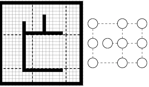
Figure 2.3: An example of graph abstraction. The grid cells are partitioned into rectangular clusters, denoted by the dashed lines.

spaces in a regular fashion, with all nodes inside a rectangle comprising a cluster, as seen in Figure 2.3. An abstraction of these clusters is produced by identifying nodes along the border of these clusters that are adjacent to other such nodes in neighboring clusters. Nodes of the abstracted graph are correlated to these cells. Edges are between all nodes common to a cluster by identifying an optimal path between these points. Valid paths are limited to those that are enclosed entirely within the cluster. The cost of the edge is defined as the cost of the optimum path between the nodes. Intra-cluster connections are defined by joining the two adjacent nodes of a cluster pair with an edge.

The resultant collection of nodes and edges produces a highly relaxed version of the original grid. This abstract grid itself can be abstracted again producing an even more abstract grid; the process could be repeated until the entire problem space is abstracted to a single node, producing a hierarchy of abstraction levels. The underlying grid is level 0 (L0). For a full detail map of the North American road

network, L0 would correspond to the individual streets. The initial abstraction is L1,

and subsequent abstractions L2, L3, and so on. This could correspond to abstractions

(31)

then countries. The topmost abstraction would encompass the entire network. Pathfinding on this hierarchy of abstractions occurs in a top-down approach. Given start and goal locations S and G, the cluster(s) they belong to are identi-fied and a path is planned between them using the edges of the abstract level. This is followed by a series of refinements as each path edge is defined by a path traversing the cluster(s) at the next lowest level of abstraction. This refinement continues down to L0.

If Sk

u is understood to be a node uin levelk, with the cost of an edge Ekuv between

u and another node v, the path for this edge on levelk₋1 can be cached.

HPA* however does not qualify as a real-time pathfinding algorithm. While the grid abstractions bring a divide and conquer approach to heuristic search, there is no constant bound on planning for any given level. At the lowest level, paths between grid clusters are still traced out with classic A*. This style of pathfinding remains subject to problem size.

2.3.1 PR LRTA*

State abstraction for real-time search was applied in [BSLY07] which introduced a new LRTA* variant called Path Refinement Learning Real-Time Search (PR-LRTS, later referred to as PR-LRTA* [BBS09]).

Instead of producing an abstraction by cutting up the L0 grid into rectangular

clusters, PR LRTA* abstracts groups of nodes by cliques of completely connected nodes, a technique described in [SB05].

(32)

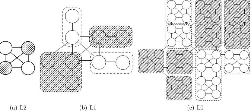
(a) L2 (b) L1 (c) L0

Figure 2.4: Corridor produced by applying LRTA* to an abstract hierarchy in PR LRTA*. A move determined by LRTA* at the top-level abstraction (a) defines a corridor for A* search at the ground-level abstraction (c).

the original search graph, with successive abstraction layers L1 and L2. If LRTA* determines a move between the two unshaded nodes in L2, this defines the unshaded corridor in L0 to define the boundary for A* search. This process repeats until the top level LRTA* search defines a corridor reaching the goal.

Real-Time performance is guaranteed the same way it is assured for LRTA*. With the LRTA* search limited to a maximum depth, an upper bound is effectively placed on the maximum size of the corridor at the ground level, regardless of the actual layout. This places a constant bound on the number of A* expansions performed at the ground level.

2.3.2 D LRTA*

D LRTA* [BLS+

(33)

de-termined though the use of a classifier. This classifier takes in information about the agent’s recent performance and makes a constant time decision as to what the depth should be. The classifier described uses several statistics easily computed in real-time, including the heuristic estimate of the agent’s current distance to the goal. Real time behaviour is assured by placing an upper bound on d′, which thus places a constant upper bound on the number of expansions for a branching factor. This is the same idea behind the real-time claims of LRTA* or PR LRTA*.

The second characteristic to D LRTA* is the use of a database to store previously computed partial solutions. Here, the problem space is abstracted to some level Ll

using a clique abstraction. Then, for each pair of l nodes, the first action to take between each is calculated and stored. Because the l nodes are an abstraction of many nodes at L0, a representative node from L0 is chosen here for its respective l

node.

2.4 Time-Bounded A*

While the introduction of abstraction hierarchies produced results with an order of magnitude improvement over LRTA*, this does come at some cost. Abstraction hierarchies are resistant to use on dynamic maps. Any change at the base grid L0 can affect edge costs for the next level, forcing re-computation of the abstract graph. In the worst case the change of a cut-edge can affect the abstraction hierarchy in its entirety. With algorithms like D LRTA*, which relies quite heavily on the off-line computation of a pattern database, extensive re-computation happens for even a single map [BBS09].

(34)

sec-tion will provide a somewhat detailed explanasec-tion of how TBA* works. As it is a recently introduced algorithm, much of the following information in this section is taken directly from [BBS09].

Algorithm 4 TBA* (start, goal, P) from [BBS09]

1: solutionF ound_←f alse

2: solutionF oundAndT raced_←f alse

3: doneT race_←true

4: loc_←start

6: if not solutionF ound then

7: solutionF ound_←A∗(lists, start, goal, NE)

8: end if

9: if not solutionF oundAndT raced then

10: if doneT race then

11: pathN ew_←lists.mostP romisingState()

12: end if

13: doneT race_←traceBack(pathN ew, loc, NT)

15: pathF ollow_←pathN ew

16: if pathF ollow.back() =goal then

17: solutionF oundAndT raced _←true

18: end if

19: end if

20: end if

21: if pathF ollow.contains(loc) then

22: loc_←pathF ollow.popF ront()

23: else

24: if loc₆=start then

25: loc_←lists.stepBack(loc)

26: else

27: loc_←loc.last

28: end if

29: end if

30: loc.last_←loc

31: moveagenttoloc

32: end while

(35)

algorithm is broken down into distinct planning and execution sections. With every iteration, lines 6 through 20 encompass the planning portion, where a round of search is carried out. Lines 21 through 31 cover the execution phase, which determines the move an agent will perform. The algorithm continues to run until the agent has reached the goal (line 5).

2.4.1 Planning

The planning portion of TBA* is broken down into two distinct steps, expansion and tracing. On line 7, expansions are performed by running A* search if the solution has not been found in some previous iteration. The parameterlistsencompasses both the open and closed lists, which are reused across iterations to facilitate global search. If A* finds the goal, this is recorded and search is suspended for subsequent iterations, if any.

Lines 9 through 19 handle the generation of paths for the agent to follow. On the first iteration, the most promising node on the open list - the node that will be expanded next when A* resumes - is used to begin tracing a path on line 13. Paths are constructed by following the parent references of each node until the starting node is reached, or the node where the agent is currently located.

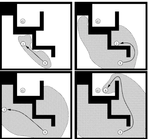
Tracing a path may take multiple iterations. When a path is traced out, it becomes the current path an agent is following (line 15). The process repeats until a path ending at the goal is traced out. Figure 2.5 shows an example of the different paths TBA* can produce for a search.

To claim real-time performance, there must be a limit on the amount of planning in a given iteration. In TBA* one of the parameters defined is theresource limit,R¶.

R is broken down into limits on the amount of work allocated per iteration to node expansion and path tracing respectively. The limit on the number of expansions (NE)

¶_R_{is never given a unit definition in the paper, but it generally understood to represent the effort}

(36)

Figure 2.5: A depiction of successive subgoals for Time Bounded A* at different intervals. Each number represents the node returned from mostPromisingState, along the search fringe at that point with the arrow being the path traced to it from the start S. The algorithm terminates when the agent (not shown) arrives at the goalG. The shaded area is the area covered by the open/closed lists for that iteration. for an iteration is:

NE =⌊R×r⌋ r∈[0,1]

For example, with R = 200, and r = 0.75, NE = 150, or 150 node expansions

are performed in the A* portion of the algorithm every iteration. The remainder is allocated to performing to tracing out paths (NT), determined as:

NT = (R−NE)×c

(37)

2.4.2 Execution

The second half of the algorithm is concerned with execution, where moves are ac-tually performed by the agent in accordance with a simple rule. The agent checks if it is on the path it is currently following, if so, it takes a step along the path (line 22), otherwise it takes a step backwards (line 25). This assures that the agent will eventually return to the path that TBA* has selected for the agent to follow. Because the closed list an acyclic tree and all paths are built from this tree, if the agent keeps stepping back it is assured to eventually end up on the path it is currently set to follow.

Figure 2.6: When TBA* switches paths to a newer one, the agent may be required to retrace steps by moving backwards until it reaches the latest path. In the worst case, the agent returns to the starting node.

For clarification, it is not necessarily true that the new path TBA* that the agent backtracks towards is the same path the agent will reach and begin following. It is conceivable that TBA* will identify and trace out any number of paths while the agent is backtracking. The decision to take a step along a path or backtrack is always made relative to the current path referenced by pathF ollow.

Once the algorithm identifies a path from the starting node to the goal, no more path switching occurs. If the agent is not somewhere along this path, it will backtrack until it is, and follow this final path to the goal. The agent is guaranteed to end up on this path; in the worst case it will return to the starting node.

2.4.3 Real-Time Claim

(38)

size. In other words, the algorithm should be able to perform the same number of expansions with each successive iteration and not taking longer to do so. To do this, the authors have constant-bounded state expansion.

For A* based search, the open list is typically implemented as a priority queue using a binary heap. Nodes on the open list are prioritised based on f-score. While retrieval of the next state to expand is an O(1) operation, insertion of successors is

O(logn), with n being the number of nodes on the heap. Because n grows with the problem size, any algorithm that maintains an open list across iterations using a heap cannot be real-time.

To claim real-time, TBA* uses a variation of a data structure used in the Fringe Search algorithm [BEHS05], which is an evolution of Iterative-Deepening A* (IDA*) [Kor85]. Fringe search was focused on improving the run-time performance of IDA* type algorithms by facilitating the reuse of the open list (the search fringe) across successive iterations, negating the rework normally necessary.

Key to this algorithm was the introduction of two lists, the now and later lists, to collectively store the nodes of the Open List. Each iteration, the algorithm runs over all nodes in the now list, either deferring their expansion by moving them to the

later list, or performing an expansion, with the successors going into thelater list for the next iteration. On the next iteration, the later list is now the now. The authors mention that IDA* iterates in a left-to-right fashion, whereas A* is best-first, which requires sorting. Fringe Search can sort or partial sort by using multiple buckets for thelater list based onf-score. This notion was carried over to TBA*. Instead of now

and later buckets, TBA* uses a bucket for each f-score. These buckets are stored in a hash table, keyed by f. Add and Remove operations on these buckets are O(1).

(39)

2.5 Summary

This chapter examined several algorithms that define the current state of real-time pathfinding applied to grid-based problem spaces. Since Korf defined the area with the introduction of LRTA*, much of the work since has focused on improving the rate at which LRTA* based algorithms converge on an optimal solution. This has typically been achieved by developing variants that feature improved first-run performance. This is important in the context of video games since subsequent trials are not likely to occur, and any occurrence of poor behaviour is to be avoided if possible.

(40)

Chapter 3 Salient Search

3.1 Motivation

With TBA*, it was noticed that the agent could often spend time moving back and forth as the (current) path changes from one subgoal to another. The agent would have to backtrack in order to put itself back on a path to follow, like in Figure 3.1. If arriving on the current path requires k steps backwards, those k steps add to the total travel cost of the agent without necessarily moving the agent any closer to the goal. This increases theTravel Ratio of the search, work the agent is performing that adds up above the cost from the start to the goal.

Salient Search began with the following idea: at time t, the agent may be closer to the goal than the cost of that return trip to follow the optimal path found forS, G. Since the cost is already expended by the agent to reach its current location, it may be cheaper to move forward if such a path exists and can be found in time. This is like the expression ‘the point of no return’.

(41)

Figure 3.1: Each successive path shares no common section with the previous one. The agent will likely have to backtrack to the start.

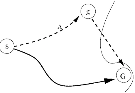
it is possible that there is a path from g to the goal that is short enough that, if known about, is more desirable than backing up. In other words, if A _→ g _→ G _≤ A_→S _→G, backing up is undesirable.

Finding such a path requires search. However, search is halted when the goal is found. Also, since TBA* is running A* search, it is known that A* finds the optimum path before any other. A* on its own will not find a path through g first.

(42)

Figure 3.2: The agent is moving towards g when a solution is found. In TBA*, the agent backs up along the path A _→ S _→ G. However, it may be desirable to move

A_→g _→G.

search order, a solution passing through g will not be found.

As well, on harder problems or problems involving a poor heuristic, A* perfor-mance tends to degrade. The search frontier expands outward in a more uniform fashion resembling breadth-first search as the best-first strategy of A* is weighed down by many nodes sharing the same score. When this happens, the lengths of successive paths from subgoals increases more slowly. These paths are also more divergent, possibly sharing only the start as a common node. When this happens, agent behavior becomes erratic. The effect on the agent resembles more of a random walk than a real attempt to move towards the goal.

Salient Search is proposed to attempt to address this situation, by allocating search from the last subgoal, while retaining the information provided from the global search. The rationale behind this concept takes two forms.

Salient Search is Time Bounded A* with the application of two new concepts:

• An additional data structure to allow us to define the salient and force search to occur along its fringe.

(43)

3.1.1 Why ‘Salient’ Search

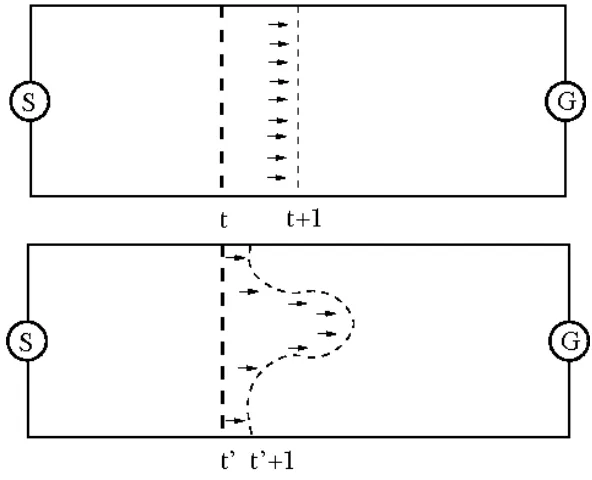
The use of the word salient is derived from the military notion of the phrase, where it describes a projection into enemy territory along a front line, a spot in the topology of the battlefield where a force has broken through the front to advance towards some objective. Comparatively, in pathfinding the progression of search using a consistent heuristic can be visualised with contour lines [RN03], and a contour defined by the Open List of a search, which is sometimes called a fringe. The analogy here is as follows: A* search produces a series of contours as search progresses. Salient Search breaks through the contour by performing search at one point of the contour, producing a salient.

Figure 3.3: A visual representation of a salient applied to heuristic search. The salient is the bulge of explored space beyond the border that would be defined once timet+1 is reached.

(44)

seen progressing as a straight line sweeping across this corridor at the top of the figure. As the algorithm iterates from timet to time t+ 1, this sweep line has moved forward, much like an army moving a front line forward with a collective advance. Eventually, this line reaches the end as the goal is reached and a path can be traced back.

With Salient Search however, the normal progression is interfered with. In the bottom portion of Figure 3.3, at time t a point along the fringe is chosen, and in the next iteration work is applied to expand this node and its successors. As a result, space that may not have been searched out by timet+ 1 instead has been, distorting the normal progression of search. This is illustrated with the search line reaching past the original A* line in one area. This is the salient: attention was focused at one point to move the frontier beyond where it would be expected to be. This comes at the expense of other areas, where the line is not as far to the right as it would otherwise be.

3.2 Salient Expansion

Applied to our real-time pathfinding algorithm, the salient itself begins as a single node in the search space. Recall that TBA* builds a path by choosing a suitable candidate from the open list, with themostP romisingStatefunction, which becomes the endpoint of said path. The salient begins from this same node. Every time a salient is initially defined, it begins with this single node, which we term the salient root. But where the path is built by backtracking through the search tree, thesalient

is defined by moving deeper through the growing search tree.

(45)

from the successors of previous nodes - until a new root is defined, at which point membership in the salient is no longer defined. Subsequent additions to the salient begin from the new root.

The salient list then is to be understood as all nodes currently on the open list that are descendents of the current salient root. Salient expansion is conducted with every node expansion when the node is itself on the salient.

Algorithm 5 shows pseudocode of the Salient Search algorithm. This is the same as TBA* in Algorithm 4. However, two lines are changed. On line 7, the A* search has been replaced with a version called SalientA*, which takes in an additional parameter. The other change is on line 11. In TBA*, pathNew was set to the head node of the Open List. Here, a function is called that takes in a strategy parameter.

A node on the open list is chosen as the salient root on line 11 of Algorithm 5. At this point, the salient is the root itself. When this node is expanded, it is removed from the open list, and its successors (if any) are now members of the salient when they are inserted onto the open list. This is true for their successor nodes, and so on. The definition of the salient in this way is illustrated in Figure 3.4.

These expansions happen up to NS times. NS itself is described in 3.2.1. The

remaining work is done following the order dictated by the open list. If a node to be expanded normally is referenced in the salient, it is treated like a salient node as a means of preserving the structure of the salient - its successors are placed onto the salient list.

3.2.1 The Salient List

(46)

(a) (b)

(c)

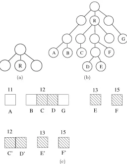
Figure 3.4: The salient on the search tree. At some point R is chosen as the salient root when R is in the open list for the tree on the left. From then on, all successors of R on the open list define the border of the salient. If nodes A through G are the open list, then the salient is defined by _{C,D,E,F_} in the tree on the right. The bottom portion illustrates what the open and salient lists look like at this point, with each set of blocks corresponding to a bucket, and the number above each being the f scores (and hash key of the bucket) of the nodes therein.

are notated with the same f scores as the parent bucket they contain references for. For the open list, node order within a particular bucket is dictated by insertion order. This is because the bucket itself is implemented as a queue†_.

(47)

Algorithm 5 Salient Search (start, goal, P)

1: solutionF ound_←f alse

2: solutionF oundAndT raced_←f alse

3: doneT race_←true

4: loc_←start

6: if not solutionF ound then

7: solutionF ound_←SalientA∗(lists, start, goal, NE, NS)

8: end if

9: if not solutionF oundAndT raced then

11: pathN ew_←lists.nextSubGoal(loc, strategy)

12: end if

13: doneT race_←traceBack(pathN ew, loc, NT)

15: pathF ollow_←pathN ew

16: if pathF ollow.back() =goal then

17: solutionF oundAndT raced _←true

18: end if

19: end if

20: end if

21: if pathF ollow.contains(loc) then

22: loc_←pathF ollow.popF ront()

23: else

24: if loc₆=start then

25: loc_←lists.stepBack(loc)

26: else

27: loc_←loc.last

28: end if

29: end if

30: loc.last_←loc

31: moveagenttoloc

32: end while

Ordering

(48)

Algorithm 6 SalientA∗₍_{lists, start, goal, N}

E, NS)

1: i_←NS

2: goalF ound_←f alse

3: while i >0 andsalientList is not empty and not goalF ound do

4: i_←i₋1

5: if salientList.next() =goal then

6: goalF ound_←true

7: end if

8: expandSalient()

9: end while

10: for remaining NE −NS+i and notgoalF ound do

11: goalF ound_←A∗

12: end for

Algorithm 7 expandNext()

1: next_←openList.next()

2: if salientList.contains(next) then

3: expandSalient()

4: else

5: move nextto closedList

6: for successor in next.successors()do

7: if not closedList.contains(successor) then

8: updateOrInsert(successor)

9: end if

10: end for

11: end if

placed onto the same global closed list.

(49)

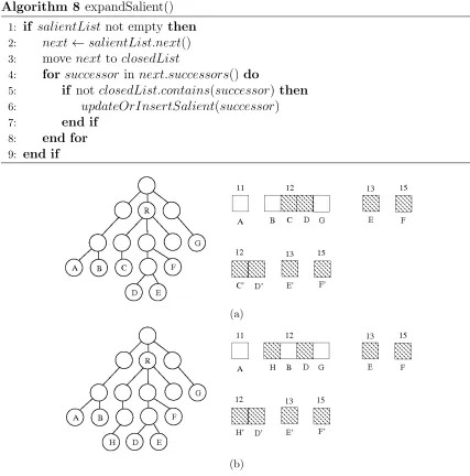
Algorithm 8 expandSalient()

1: if salientList not empty then

2: next_←salientList.next()

3: move nextto closedList

4: for successor in next.successors()do

5: if not closedList.contains(successor) then

6: updateOrInsertSalient(successor)

7: end if

8: end for

9: end if

(a)

(b)

Figure 3.5: The next node to be expanded by salient expansion is always identified by the head of the salient list. Here it is node C. It is removed from the open list, and its successors are put into both lists in the preferred order.

In TBA*, nodes are only removed from the open list in best-first order. In Salient Search however, the best of the salient may be located in a different location.

(50)

even if a consistent heuristic is being used since Salient Search does not follow A*’s expansion order globally‡_.

With a heap based open list, this would involve updating the node’s key, a Θ(logn) operation. However, because the open list in this algorithm uses constant time (O(1)) operations for adding and removing nodes, those operations can be used to achieve an update.

Thus, with all actions appropriately mirrored on the salient list, it is assured to be a subset of the open list with the following properties:

• All nodes on the salient list are descendents of the salient root

• All descendents of the salient root that are on the open list are also in the salient list

• The salient list maintains the same ordering as the open list

3.2.2 Allocating Work - N

S

To control the amount of expansion limited to the salient, a new parameter is in-troduced. NS controls the number of expansions per iteration that are allocated to

ensuring work is done in the salient, being a value 0 _≤S _≤ E. Any remaining work is used to perform expansions as normal by the ordering of the open list.

A particular value for NS however is not a guarantee that NS salient expansions

will be performed. First, if the salient list is exhausted, then salient expansion obvi-ously cannot be performed. This is possible if for example the salient root expands into a closed off space search and is exhausted within it. Secondly, through regular expansion, a salient node could be selected for expansion through regular A* search when the node is at the top of the lowest scored bucket. If this occurs, it is treated as a salient expansion, with successors being placed on the salient list (Algorithm 7,

(51)

lines 2-3). Detecting this is a trivial operation because the node will be at the head of both the open and salient lists. With these two situations, the number of salient expansions in any given iteration can exceed or be less than NS.

When NS is 0, no action will be taken to perform node expansions out of order,

effectively turning off salient expansion. Search will proceed exactly as it would in TBA*. That is to say, the planning portion of the algorithm will remain unchanged, proceeding in the same way A* does. This is not to say that the salient will not exist. The definition of the salient list is maintained from R like in Figure 3.4, there is simply no explicit allocation of work to produce successors from the members of this list. The list remains maintained for use with the strategy, which is described in Section 3.3. Strategies affect the choice of paths, so even with search proceeding exactly as it would under TBA*, Salient Search can result in different behaviour for an agent given the same problem.

3.3 Subgoal Selection by Strategy

Recall that TBA* produces paths by choosing a subgoal. These subgoals are always the most promising node currently residing on the open list. This subgoal becomes the endpoint of a new path. As long as this node is not the goal, search will continue, because the subgoal is always the next node to be expanded. This remains true in Salient Search. But, the salient list now provides additional information regarding this decision. We know which nodes are descendents of the path that has just finished being traced back, allowing us to know if a prospective subgoal will produce a path which lengthens the current one. This information can be used to modify the selection of a subgoal; the decision can be made to instead selected the most promising node of the salient list instead.

(52)

other parameters necessary, and returns which one will serve as the next subgoal. The decision will decide not only if the next path is an extension of the current one, but also whether the new salient will be an extension of the current salient.

Trivially, if the salient list is empty or the head of the salient list is the same node as the head of the open list then the decision is moot. The only other restriction on a strategy is that it satisfies the realtime requirements.

What follows are two example strategies. The first is a simple tie-breaking strategy for nodes with the same f score. The second strategy makes use of the agent’s location.

3.3.1 Simple Tie-Breaking

In theTie-Breaking (TB) strategy, the preference for a subgoal with the bestf score remains the same. However, as mentioned in 3.2.1, the salient list allows constant time determination of whether a potential subgoal extends the current path. Extending the current path means the agent will not require backtracking if it is following the current path. Given the lack of sorting between all nodes with the same f-score, we can use this information to choose a subgoal. If the head nodes of lists arenOpen and

nSalient respectively, the strategy is:

T B(nOpen, nSalient) =

  

 

nOpen, if f(nOpen)< f(nSalient)

nSalient, Otherwise

Since by definitionnOpenis the head of the lowestf-bucket on the open list,nSalient

will be in the same bucket, or have a higher f-score. Because the salient list has the same ordering as the open List, nOpen is not a descendent of the (current) subgoal

(53)

3.3.2 Agent Heuristic Distance

In theAgent Distance (AD) strategy, the heuristic used in planning is used to answer the question of which subgoal is closer to the agent at that point in time. The heuristic estimates are taken, and the subgoal with the lower distance is chosen.

AD(loc, nOpen, nSalient) =

  

 

nOpen, if h(loc, nOpen)< h(loc, nSalient)

nSalient, Otherwise

The rationale behind this strategy is that a goal that is farther away from the agent will take longer to reach, increasing the likelihood that movement towards the subgoal will be wasted effort when the subgoal again changes.

Heuristic distance is used because discovering the actual travel distance is an application of the Lowest Common Ancestor (LCA) problem. The traversal involves backtracking from the current agent location A to the lowest common ancestor C, and then forwards to the desired subgoal ng. The total cost would correspond to:

T ravelCost(A, ng) =g(A) +g(ng)−2g(C)

No constant time solution exists to identify C. In the general case, finding a solution takes O(h) where h is tree height§_{. Constant time queries can be devised}

but this requires anO(n) scan of the tree, which is unfeasible with the lists (and thus the trees) in constant flux as they grow. Work on the LCA problem can be found in [HT84, AHU73, BFc00].

(54)

3.4 Summary

In this Chapter the Salient Search Algorithm was introduced. Salient Search is a vari-ation of Time Bounded A* that attempts an opportunistic tradeoff between planned solution quality and the realised agent path. Salient Search differs from TBA* by using a salient list to maintain an ordered reference to all descendents of the current subgoal. Salient Search uses this list to conductSalient expansion - deliberate search from the current subgoal.

(55)

Chapter 4 Experimental Setup and Analysis

The following chapter will provide an empirical analysis of the Salient Search algo-rithm.

4.1 Problem Domain

All testing is done in the domain of two-dimensional grids. For real-time algo-rithms, grid-based testing has been used since at least early work on LRTA* [IK91], and remains a popular choice for testing pathfinding algorithms in recent literature [BBS09, BSLY07, Stu07, ZSH+

09, SYCK09].

In this thesis, we used a collection of grid-based maps taken from a collection of video games. These are taken from a larger collection of maps taken from the Hierarchical Open Graph (HOG) Framework [Stu10]. The appeal of using these maps is they are sourced from several real successful computer games, adding practical appreciation to the results. This set is also utilised in other literature [BSLY07, BB09, BEHS05], including Time Bounded A* [BBS09].

(56)

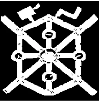
Figure 4.1: AR0701SR, an example map (derived from [Stu10, CSE00]) representations can be found in Appendix B.

All maps are scaled to 320x320 cells in size. Scaling was accomplished by taking a bitmap representation of the problem space† _{and resampling to the target dimensions}

via nearest neighbour interpolation. For scaling up to a larger size this resampling technique preserves the graph homomorphism. The cells themselves are all in one of two states: either freely traversable by an agent or blocked.

Figure 4.2: Different grid types. Left: The Cardinal grid. Right: The Octile grid The maps themselves merely describe blocked and unblocked spaces. Also needed is a description of legitimate moves the agent can perform, which are described by a topology. Two different grid topologies were used in this experiment: cardinal and octile.

(57)

In a cardinal grid, there are only 4 possible moves from a given grid cell, up, down, left, and right. The octile grid is an extension of this by allowing moves in diagonal directions. These types can be seen in Figure 4.2. On the cardinal grid, all moves incur a cost of 1. On octile grids, this is the same for cardinal moves. However, diagonal moves are assigned a cost of √2‡_.

It is worth testing with differing topologies because each produces a different effective branching factor, which directly influences the rate of growth of the search space. This in turn can influence the effectiveness of some pathfinding algorithms, with some algorithms outperforming others for a given topology. Further reading on this can be found in [Yap02, BEH+

03].

Figure 4.3: An illustration of corner cutting. The dashed lines on the left show valid moves on the grid. An agent cannot move diagonally if doing so would cross a corner of the grid shared by a blocked cell. If corner cutting is allowed, an agent could move ‘through’ the blocked cells in the example on the right.

Diagonal moves have an additional constraint. They are only permitted if the neighbour(s) common to both cells of the move are unblocked. This situation is commonly known as corner cutting. This also means that a diagonal move is only allowed if moving to the node can be made with two sets of cardinal moves. See Figure 4.3. While there are computer games that permit corner cutting for their agents (e.g. [GG05]), other literature tends to forbid it, so we have done the same.

(58)

4.1.1 Assumptions

There are several assumptions in the testing environment that should be noted: 1. Both Time-Bounded A* and Salient Search are episodic. There are no trials or

convergence process as with the LRTA*-based approaches; subsequent runs of either algorithm on the same problem do not influence performance, as no infor-mation is preserved once the algorithm completes. Thus there is no utilisation of any database of partial or complete solutions for any search instance.

2. The problem environment is static§_{, not dynamic. Cells do not transition}

be-tween a blocked or unblocked state. Similarly, edges bebe-tween grid cells are not added or removed, and the cost incurred moving between cells does not change. 3. Each search is single-agent. Multiple agents are not conducting search

simulta-neously on a common map.

4. All maps keep the safety assumption. From [BBS09]: “The goal state can be reached from any state reachable from the start state”. In fact, the maps used have been modified where necessary to prevent any ‘islands’, so every unblocked state is reachable by every other unblocked state. This was verified by running a breadth-first search with duplicate detection over each map and checking that every unblocked cell was visited by the search.

5. There is nofreespace assumption as it appears in algorithms like RTAA*. Node expansion involves the true state and cost on the map, not open space beyond a search horizon perceived by an agent. Rather, search proceeds with perfect information of the map.

§_{Technically, Time Bounded A* and Salient Search’s agent can be said to inhabit a}_semidynamic

environment. Since the agent is potentially incurring a nonzero travel cost with every step before

(59)

4.1.2 Search Pair Generation

For each of the 50 maps, start and location pairs were generated. Classic A* was run between these points to determine an optimal path between these points, and the pair was kept if the path found by the search had a cost between 50 and 500. This was repeated until 100 pairs were generated for each map, for a total of 5000 problems. A particular coordinate could be used as a start or goal location in multiple problems, and there was no prohibition against a particular pair used in reverse. This process was repeated separately for each of the grid topologies.

4.1.3 Heuristics Used

A separate heuristic was used for each of the grid topologies. Each heuristic is consid-ered perfect in an unblocked grid of its type. With no obstacles, the heuristics used give the true cost h∗ between the start and goal locations.

Cardinal Maps

The Manhattan heuristic¶ _{is the sum of the distance between two points along the}

axis of each dimension. In a two dimensional grid world it is simply:

M anhattan : ∆x+ ∆y

Octile Maps

For octile grids the heuristic of the same name is used: a cost of 1 for NSEW moves, and√2k _{for diagonal moves. Because the agent can move in both}_x_and _y_dimensions

in a single step, the heuristic is the minimum number of diagonal steps to finish moving in one dimension, plus the remaining number of steps to complete travel in

¶_{May also be referred to as the}_Cardinal _or_Taxi-cab _or_{City block} _distance.

(60)

the remaining dimension. In equation form, this is:

Octile: min(∆x,∆y)_×√2 +_|∆x₋∆y_|

For the given topology, the same heuristic was used regardless of the particular algorithm (A*, TBA*, or SS) being run.

4.1.4 Parameters

As described in [BBS09], the parameter NE is defined as a ratio of the resource limit

R by NE =⌊R×r⌋, wherer ∈[0,1]. The authors elected to fixr at 0.9, and we have

done the same for our experiment. As well, the parameter cis fixed at a value of 10. The values of the resource limit (R limit) used in the experiments were R =_{25, 50, 100, 500, 1000_}.

Table 4.1: NS expansion by percentage of NE, r= 0.9

R Limit

% 25 50 100 500 1000 30 7 13 27 135 270 50 11 22 45 225 450 75 16 34 67 338 675

NS, the parameter used to control the number of expansions inside the salient,

took on values corresponding to 30%, 50% and 75% of the value of NE. The number

of expansions this corresponds to for each permutation can be found in Table 4.1. For example, With an R limit of 50, there will be 45 expansions in an iteration, and if 30% should be directed towards the salient, NS takes on a value of 13.

For Salient Search’s strategy parameter, both the Agent Distance (AD) and Tie-Breaking (TB) strategies described in 3.3 were tested for each NS/R limit

(61)

Thus, with 5000 different searches across the 50 maps, there are 25000 datapoints created using TBA* (5000 problems _×5 R Limits), and 150000 using Salient Search (5000 problems _× 5 R Limits_× 3 Salient expansion settings _× 2 strategies).

4.2 Results

All experimental results were collected using the same hardware and environment for both TBA* and Salient Search. The hardware was an IntelRCoreTMi5 750 CPU

at 2.67GHz with 4GB of RAM installed. The operating environment was the 64bit edition of Windows 7 Professional. All test code including the algorithms under test were implemented in the C# language, targeting version 3.5 of the .NET Common Language Runtime. Figures and tables regarding the results and statistical analysis of the experiments were created using the R programming language environment [R D10] using the Rcmdr package [Fox05].

A* Solution Cost − Octile Maps

Solution Cost

Frequency

100 200 300 400 500

0 200 400 600 800 1000 (a)

A* Solution Cost − Cardinal Maps

Solution Cost

Frequency

100 200 300 400 500

0 200 400 600 800 (b)

Figure 4.4: Histogram of A* costs for different map styles

Salient Search

Scholarship at UWindsor

Scholarship at UWindsor

Salient Search

Salient Search

Author’s Declaration of Originality

Abstract

Dedication

Acknowledgements

Table of Contents

List of Tables

List of Figures

List of Algorithms

Glossary

Chapter 1

Introduction

1.1

Problem Domain

1.2

Contribution of this Thesis

1.3

Organization of this Thesis

Chapter 2

Real-time Pathfinding

2.1

A*

2.2

Learning Real-Time Algorithms

2.2.1

LRTA*

2.2.2

K LRTA*

2.2.3

LRTA*(k)

2.2.4

RTAA*

2.2.5

P-LRTA*

2.3

Hierarchical Real-Time Algorithms

2.3.1

PR LRTA*

2.3.2

D LRTA*

2.4

Time-Bounded A*

2.4.1

Planning

2.4.2

Execution

2.4.3

Real-Time Claim

2.5

Summary

Chapter 3

Salient Search

3.1

Motivation

3.1.1

Why ‘Salient’ Search

3.2

Salient Expansion

3.2.1

The Salient List

3.2.2

Allocating Work - N

3.3

Subgoal Selection by Strategy

3.3.1

Simple Tie-Breaking

3.3.2

Agent Heuristic Distance

3.4

Summary

Chapter 4

Experimental Setup and Analysis

4.1

Problem Domain

4.1.1

Assumptions