Evaluation and Hardware Realization for a Face Recognition System

(1)

University of Windsor University of Windsor

Scholarship at UWindsor

Electronic Theses and Dissertations Theses, Dissertations, and Major Papers

2013

Evaluation and Hardware Realization for a Face Recognition

System

Kaushik Ray

University of Windsor

Follow this and additional works at: https://scholar.uwindsor.ca/etd

Recommended Citation Recommended Citation

Ray, Kaushik, "Evaluation and Hardware Realization for a Face Recognition System" (2013). Electronic Theses and Dissertations. 4923.

https://scholar.uwindsor.ca/etd/4923

This online database contains the full-text of PhD dissertations and Masters’ theses of University of Windsor students from 1954 forward. These documents are made available for personal study and research purposes only, in accordance with the Canadian Copyright Act and the Creative Commons license—CC BY-NC-ND (Attribution, Non-Commercial, No Derivative Works). Under this license, works must always be attributed to the copyright holder (original author), cannot be used for any commercial purposes, and may not be altered. Any other use would require the permission of the copyright holder. Students may inquire about withdrawing their dissertation and/or thesis from this database. For additional inquiries, please contact the repository administrator via email

(2)

Evaluation and Hardware Realization for a Face Recognition System

By

Kaushik Ray

A Thesis

Submitted to the Faculty of Graduate Studies through Electrical and Computer Engineering in Partial Fulfillment of the Requirements for

the Degree of Master of Applied Science at the University of Windsor

Windsor, Ontario, Canada

2013

(3)

Evaluation and Hardware Realization for a Face Recognition System

by

Kaushik Ray

APPROVED BY:

______________________________________________ Dr. Shaohong Cheng, Outside Dept. Reader Department of Civil and Environmental Engineering

______________________________________________

Dr. Mohammed A. S. Khalid, Internal Dept. Reader

Dept. of Electrical & Computer Engineering

______________________________________________ Dr J. Wu, Advisor

Dept. of Electrical & Computer Engineering

(4)

iii

Co-Authorship Declaration

I hereby declare that this thesis incorporates material that is result of joint

research, as follows:

This thesis also incorporates the outcome of a joint research undertaken in

collaboration with Ashirbani Saha under the supervision of Professor Jonathan

Wu. The collaboration is covered in Chapter 3 of the thesis. The experimental

designs, data analysis and the hardware design were performed by the author.

The contributions of co-authors were primarily through the face recognition

algorithm idea and implementation, provision of proof reading and reviewing the

research paper regarding the technical content.

I am aware of the University of Windsor Senate Policy on Authorship and I certify

that I have properly acknowledged the contribution of other researchers to my

thesis, and have obtained written permission from each of the co-authors to

include the above materials in my thesis.

I certify that, with the above qualification, this thesis, and the research to which it

refers, is the product of my own work.

I declare that, to the best of my knowledge, my thesis does not infringe upon

(5)

iv

techniques, quotations, or any other material from the work of other people

included in my thesis, published or otherwise, are fully acknowledged in

accordance with the standard referencing practices. Furthermore, to the extent

that I have included copyrighted material that surpasses the bounds of fair

dealing within the meaning of the Canada Copyright Act, I certify that I have

obtained a written permission from the copyright owner(s) to include such

material(s) in my thesis.

I declare that this is a true copy of my thesis, including any final revisions, as

approved by my thesis committee and the Graduate Studies office, and that this

thesis has not been submitted for a higher degree to any other University or

(6)

v

Abstract

Facial recognition from an image or a video sequence draws attention for many

image processing researchers owing to its myriad applications in real world as

well as in computer vision, human-computer interaction and intelligent systems.

Facial structures have unique features which can be extracted using some

mathematical tools. We have used Principal Component Analysis (PCA) and Local

Binary Pattern (LBP) to extract them and stored them in a database. When the

query image is given the facial features are extracted and compared to the

previously obtained results using Sparse Face recognition. Detailed test methods

have been defined and an extensive testing of the algorithm has been performed

on various standard databases. The results have been tabulated with required

graphs. The proposed algorithm has been compared to other different algorithms

which show significant improvement in results with small number of training

samples. Finally the algorithm was integrated in a hardware system so that it can

(7)

vi

to my

(8)

vii

Acknowledgements

I express my sincere gratitude to my adviser, Dr. Q.M. Jonathan Wu for giving me

the opportunity to work under his supervision as well as for his constant guidance

and support. I would like to thank Mr. Frank Cicchello for his valuable suggestions

and comments. I would like to thank Ashirbani Saha and Dibyendu Mukherjee for

all their constant guidance, help and motivation during my research work.

I am thankful to my friends and colleagues, in particular Charrie, Carolyn, Conrad,

Carina, Candace, and Gaurav for their help and frequent assistance and

motivation throughout my work and stay. Last but not the least, I would like to

thank my mom, dad and my sister for their love and support which motivated me

(9)

viii

List of Tables

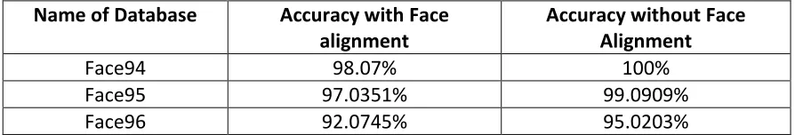
Table 3.1: Change in percentage accuracy with and without the alignment.

Table 3.2: Different images used for training and testing from Face 94 database.

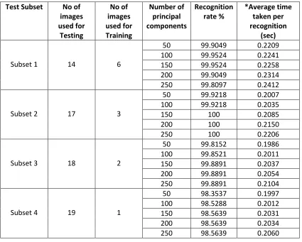
Table 3.3: Results from Procedure 1 on Face 94 database.

Table 3.14: Different images used for training and testing from FEI face database.

Table 3.15: Results from Procedure 1 on FEI face database for subject 1 to 100.

(15)

xiv

Table 3.17: Different images used for training and testing from FEI face database.

Table 3.20: Different images used for training and testing from JAFFE database in

different Subsets.

Table 3.21: Results from Procedure 1 on JAFFE database.

Table 3.22: Different images used for training and testing from JAFFE database.

Table 3.23: Results from Procedure 2 on JAFFE database.

Table 3.24: Different images used for training and testing from PUT Vein Pattern

database in different Subsets.

Table 3.25: Results from Procedure 1 on PUT Vein Pattern database.

Table 3.26: Different images used for training and testing from PUT Vein Pattern

Table 3.27: Results from Procedure 2 on PUT Vein Pattern database.

Table 3.28: Shows the different images used for training and testing the Yale Face

Table 3.29: Results from Procedure 1 on Yale Face database.

Table 3.30: Shows the different images used for training and testing the Yale Face

Table 3.31: Results from Procedure 2 on Yale Face database.

Table 3.32: Tablets the results obtained for facial recognition algorithms on

different databases and compared it to SFRLBP

Table 3.33: Tabulates results for face recognition with different listed algorithms

and the accuracy obtained for Yale face database.

Table 4.1: lists all the components on the board marked in Figure 4.5.

Table 4.2: Lists the function of each pin in a 20 x 4 LCD.

(16)

xv

(17)

xvi

List of Figures

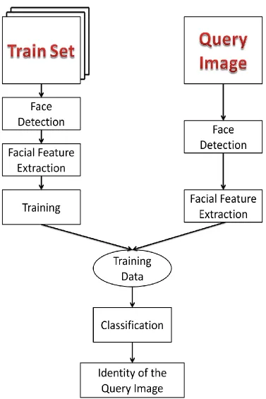
Figure 2.1: General workflow of a face recognition system.

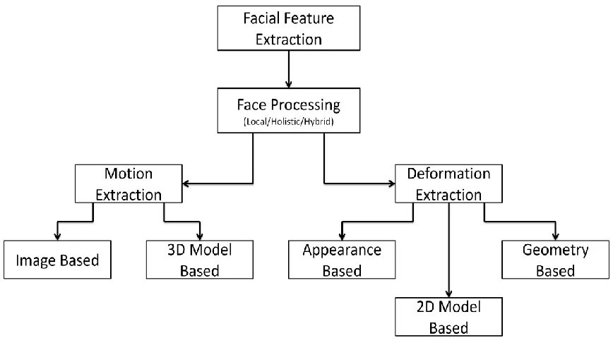
Figure 2.2: Different type of facial feature extraction approaches.

Figure 3.1: Shows the basic blocks and the process flow of the proposed facial

recognition algorithm.

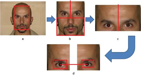
Figure 3.2: Alignment process flow.

Figure 3.3: (a) Shows the holes present due to the rotation of the image marked

by red circles. (b) Shows the image processed with a bilinear filter.

Figure 3.4: The Basic LBP operator.

Figure 3.5: A sample image set from Face 94 database.

Figure 3.6: Graphs showing accuracy in percentage against the number of

Principle Components.

Figure 3.10: Graphs showing accuracy in percentage against the number of

(18)

xvii

Figure 3.14: Some examples of image variations from the FEI face database.

Figure 3.15: In this figure, 2 sets of five images have been shown which were used

to test and train the algorithm from FEI Face Database.

Principle Components for Set 1.

Figure 3.20: A sample image set from JAFFE database.

Figure 3.23: In A sample image set from PUT Vein Pattern database.

Figure 3.26: 2 sets of five images have been showed which were used to test and

train the algorithm.

(19)

xviii

Figure 3.29: Shows two sample images from PUT Vein Pattern Database.

Figure 4.1: The following figure shows the major three blocks of the proposed

system.

Figure 4.2: Shows the camera module with the IR LED’s mounted to it.

Figure 4.3: Shows images captured in different lighting conditions.

Figure 4.4: This diagram shows the basic blocks of the GUI and the IR intensity

controller.

Figure 4.5: This picture shows the main board.

Figure 4.6: A simple circuit diagram for 7805 has been displayed in the above

figure.

Figure 4.7: A 20×4 LCD display module.

Figure 4.8: Circuit diagram showing the basic wiring for a LCD module.

Figure 4.9: A picture of the keyboard used for the GUI Design.

Figure 4.10: Displays the pin out of a AT24C64 EEPROM.

Figure 4.11: Shows the pin out and the basic circuit diagram for a MAX 232.

Figure 4.12: This graph shows the illumination verses current output in for

BPW34 sensor.

Figure 4.13: The above picture shows the BPW34 sensor.

Figure 4.14: In this diagram we have a simple design showing a current to voltage

convertor with D1 as the BPW34.

Figure 4.15: Shows the pin out for the opamp.

Figure 4.16: Pin diagram of an AtMega 32 controller.

Figure 4.17: The basic circuit diagram of an AtMega 32 controller.

(20)

xix

Figure 4.19: Displays a picture of the main processing board.

(21)

xx

List of Acronyms

AAM Active Appearance Method

ADC Analog to Digital Converter

ASCII American Standard Code for Information Exchange

ASIC Application-Specific Integrated Circuit

ASIP Application Specific Instruction set Processor

ASM Active Shape Model

ASSP Application Specific Signal Processor

BJT Bipolar Junction Transistors

CCD Charged Coupled Device

CMOS Complementary Metal-Oxide Semiconductor

CMRR Common Mode Relation Ratio

CPU Central Processing Unit

CUDA Compute Unified Device Architecture

DAQ Data Acquisition

DCT Discrete Cosine Transform

DSP Digital Signal Processors

(22)

xxi

EBGM Elastic Bunch Graph Matching

ED Euclidean Distance

EEPROM Electrically Erasable and Programmable Read-Only Memory

FFT Fast Fourier Transform

FPGA Field Programmable Gate Array

GB Gigabyte

GND Ground

GPIO General Purpose Input/Output

GPP General Purpose Processors

GPU Graphics Processing Unit

GUI Graphical User Interface

HD Hamming Distance

HEX Hexadecimal

HMM Hidden Markov Model

HSD Haar Spectral Diagram

IC Integrated Circuits

IDE Integrated Drive Electronics

IO Input/Output

IR Infra-red

JAFFE Japanese Female Facial Expression

JTAG Joint Test Action Group

KB Kilobyte

KN Known Neighbor

(23)

xxii

LCD Liquid Cristal Display

LDA Linear Discriminant Analysis

LED Light Emitting Diode

LSB Least Significant Bit

MB Megabyte

MHz Megahertz

MIPS Million Instructions Per Second

OMP Orthogonal Matching Pursuit

OS Operating System

PC Personal Computer

PCA Principal Component Analysis

PDIP Plastic Dual In-line Package

PWM Pulse Width Modulation

RAM Random Access Memory

RBF Radical Based Function

RC Resistance and Capacitance

RGB Red Green Blue

RISC Reduced Instruction Set Computing

ROM Read-Only Memory

RX Receive

SCL Serial Clock

SD Secure Digital

SDA Serial Data

(24)

xxiii

SoC System on Chip

SRAM Static Random Access Memory

STFT Sort-Time Fourier Transform

SVM Support Vector Machine

TTL Transistor-Transistor Logic

TX Transmit

UART Universal Asynchronous Receiver/Transmitter

USB Universal Serial Bus

VI Voltage Input

VO Voltage Output

WP Wright Protect

(25)

1

Chapter 1: Introduction

The primary objective for this thesis is to explain our proposed algorithm, design,

application and tests for a robust face recognition algorithm and to explain how this

system can be implemented onto hardware in order to realize its portability,

surveillance potential to solve problems involving automotive theft and driver

authentication. We believe this design conception will produce striking results as well

as a critical, distinguished, state-of-the-art product.

1.1 Why use face recognition software?

Every day, thousands of terabytes of images around the world are captured in the form

of videos from surveillance cameras. Of those captured images, 95 percent consist of

facial data, so finding a correct algorithm to extract these facial structures and index

them for facial recognition is vital. Presently, there are a myriad of applications for a

robust face detection and recognition model. These applications are not only crucial

within the theoretical world, but they have a gargantuan significance in the real world.

For example, accurate facial recognition can be used for identification of criminals, for

(26)

2

feature-length films, for use by investigators, scientists and engineers in the fields of

human computer interaction and homeland security and for key barriers to automotive

theft.

1.2 Challenges

Over the years, researchers have faced serious challenges with facial recognition

systems. Although in the past few years we have seen significant improvement, most of

the face recognition algorithms work well only with frontal faces. Occlusion of the face

due to sunglasses, long hair, or some object that partially covers the face has made the

production of a reliable face recognition system challenging. In addition, change in

facial expression, low light, and low resolution pictures have proved detrimental for a

trustworthy, consistent face recognition product. Difficulties with robustness verses

processing speed have made the manufacture of this crucial recognition system even

more arduous.

1.3 Motivation

The challenges mentioned in section 1.2 make face recognition one of the major

research topics in computer vision. Face recognition being one of the diverse research

topic with a lot of developments and new algorithms proposed every day but in

retrospect that fact there are major gaps to be filled up for a perfect design. Everyday

researchers are trying to fill these gaps and find a better solution. A trade-off between

the speed and accuracy looms large as the primary research focus. Algorithms with

(27)

3

complexity have lower accuracy. One of the other major motivational factors is a

Waterloo based company brought into focus for a requirement of a portable device

capable of face recognition. The primary objective for the device is to be installed in a

car for authentication of the eligible drivers.

1.4 Objective

The objective for the research detailed in this thesis is to improve the accuracy and

speed for a face recognition system using sparse face recognition and Local Binary

Pattern or LBP. Two different test procedures are presented to test the proposed

algorithm on various standard datasets. Each of these datasets carries its own, unique

features including variations in expression, lighting conditions, partial occultation, and,

cluttered backgrounds. The final objective of this thesis is to demonstrate an available

design and execution of a face recognition system in a portable hardware which can be

used as a standalone device.

1.5 Scope

This research comprises a new approach towards face recognition with LBP and sparse

face recognition along with rigorous testing and detailed observations on various

standard datasets in order to reduce the whole system in small scale hardware and

design a standalone system. Most embedded hardware systems use Hidden Markov

Model (HMM) for embedded face recognition. This paper will present one of the first

(28)

4

1.6 Organization

This thesis has been organized as follows:

 Chapter 2 details a review of the related work involved as well as a general

workflow for a face recognition system.

 Chapter 3 specifies an overview of the present research along with required

flowcharts and diagrams. A detailed tabulation of the results obtained is

presented along with relevant graphs.

 Chapter 4 concentrates upon system miniaturization with a small sized board to

make it a portable and standalone system along with other hardware support to

assist the proposed algorithm.

 Chapter 5 discusses the future work that can be performed to make this

(29)

5

Chapter 2: Literature Review

Faces are complex multi-dimensional structures and over the past three decades, image

processing researchers have been working hard to execute a suitable procedure to

extract, analyze and recognize facial features. This system is needed to find the identity

of a test subject that will be significantly more reliable than the present systems.

Most of the early models were based on Construct Detailed models of retinal or striate

activity. It was much later, with the increase in computational power, that face

recognition turned to computational modeling. Most of these computational models of

face recognition contain some basic blocks. Many different researchers have tried

several different procedures to find a perfect algorithm to devise a facial recognition

system that will be almost perfect.

2.1 General Workflow

Most facial recognition algorithms follow a generic frame work which is presented in

Figure 2.1. The basic steps for facial recognition and some of the existing works in the

(30)

6

Figure 2.1: General workflow of a face recognition system.

2.1.1 Facial image acquisition

A face acquisition system identifies, locates and extracts features from a complex scene

with cluttered backgrounds. For a face recognition system a good face detector is very

important. There are many approaches for a face detection system - where some use an

[91][92] exact location of faces, others operate [93][94] with a coarse location of faces.

Modular eigenspace method was used by Essa and Pentland [91] for face detection.

Principal component analysis or PCA coefficients of facial images were used to extract

facial information from still images and image sequences. Hong et. al [92] used the

Pearson Spotter system [95] for tracking the head so stereo disparity, skin color

detection and convex region detector to figure out the exact face location. Methods like

Active Appearance or AAM and local motion model [93] can work with a course location

of faces. The most popular and effective face detection system used in recent research

is Viola-Jones’ face detector, which uses boosted haar features to detect faces.

2.1.2 Preprocessing of the facial image

Images captured in different resolution are computed in a uniform scale; RGB images

can be converted to gray image; grey image can be converted to binary image. Noise

reduction filter can be used or face alignment algorithm can be used for aligning the

(31)

7

2.1.3 Facial feature extraction

Feature extraction is one of the major tasks in an image processing algorithm. Feature

extraction categorizes the image into correct abstract classes relevant to the context.

Every image is a two dimensional, three dimensional or fore dimensional data set

depending on the type of image or a video sequence. The basic idea is to use some

mathematical tool on these data sets or matrices and extract meaningful information. In

Figure 2.2 we can see some methods in which face detection algorithms are broadly

classified. These methods use local information like portion of the eye or mouth [98]

[99] for extracting the facial features. Holestic methods [92] [94] [97] use the entire face

or points from different positions from the face. Methods which use both global and

local features are also in existence and are commonly known as hybrid methods [91]

[100].

Most commonly the image features are extracted in spatial domain or transform

domain. In spatial domain it mostly calculates the density of the pixel or the distance

between the lips and nose or the distance between the lips and the line joining the two

eyes, mean standard deviation etc. In transformation domain methods like Fast Fourier

Transform (FFT) [73], Discrete Cosine Transform (DCT) [74], Sort-Time Fourier Transform

(STFT) [75], Discrete Wavelet Transform (DWT) [76] etc. are some of the common

(32)

8

Figure 2.2: Different type of facial feature extraction approaches.

2.1.4 Matching the query image with the database image

While matching the query image, the features extracted from the training facial images

are stored in a database. Next the query image is compared with the images from the

database which have been processed and stored. Most common methods include

Euclidean Distance (ED), Hamming Distance (HD), Support Vector Machine (SVM) [78],

Known Neighbor (KN) [77] etc.

One of the most efficient computational models was proposed by Matthew Turk and

Alex Pentland [43] in 1991; these are known as Eigenfaces were one of the best

computational models at the time. Eigenfaces were used for a long time for face

detection and recognition, all the while yielding good results. With further research,

many drawbacks of the Eigenfaces were able to be overcome. Jeffery and Masatoshi

(33)

9

to represent the Haar spectrum of Boolean function. In 2003 Kan Ma and Xiaoou Tang

[71] proposed something similar to the Garber face graph known as Discrete Wavelet

Face Graph. Duan and Zheng [72] proposed a method which uses grey level AdaBoost

scheme for extracting Haar like features. In the next following years many new

algorithms were developed which has an upper hand on top of the previous algorithm.

Paul and Abbes [80] proposed a method to determine most discriminative coefficients

in DWT/PCA based face recognition algorithm. Jun Ying Gan and Jun Feng Liu [81]

proposed an innovative and novel approach based on wavelet features and their

algorithm is known as Kernel Fisher Discriminant Analysis [82].

In more recent years, there have been more sophisticate algorithms proposed which are

very robust and efficient. Some of the major approaches include PCA [43], Linear

Discriminant Analysis (LDA) [83], Elastic Bunch Graph Matching (EBGM) [84], LBP [9],

Sparse Representation [67] [69]. With the advent of all these new avenues, facial

recognition techniques have been going uphill and reaching towards the goal to give an

accuracy of close to 100% recognition rate. In the next following chapters we will

explore a very new and unique way of designing Face recognition systems with sparse

face recognition.

2.2 Embedded face recognition system

A Face recognition system is challenging by itself, so embedded face recognition

systems must be even more challenging. Due to lower processing power and limitation

(34)

10

the most popular embedded face recognition systems available are neural network

based face recognition systems [87]. Eigenfaces have been used for a long time; they are

known to give good results using FFT based calculations for distance measurement as

well as face detection [89], making hardware implementation easier and faster. In 2003

Fan Yang and Michel Paindavoine designed a Radical Based Function (RBF) Neural

Network for real time tracing and face recognition on embedded systems. They

implemented the same algorithm on different embedded hardware; the result and

speed varied based on the hardware used: 92 percent accuracy on Fast Programmable

Gate Array (FPGA); 85 percent accuracy on a ZISC processor [90]; and 98.2 percent

accuracy on a Digital Signal Processor (DSP). With the increase in accuracy there is a

decrease in the processing speed for the system. There are many other efforts for

embedded face recognition systems which include designing a face recognition system

by Liu et al. [84] using optical correlation technique.

In this thesis we have implemented the proposed algorithm on a portable hardware

system. This is the first approach for designing a portable face recognition system with

(35)

11

Chapter 3: Software and Algorithm

3.1 Introduction

Development of an automatic face recognition algorithm is one of the major challenges

for the image processing and pattern recognition researchers. Many algorithms have

been proposed and all has some pros and cons. Some algorithms have a high efficiency

rate but with a higher time complexity; others have a lower time complexity but with a

lower efficiency rate (i.e. Eigenfaces). The prime goal for our thesis is to find an

algorithm which can excel in two folds. In some recent research, it has been observed

that LBP can extract useful correlated information out of a facial image [44]. We have

used the same to design an algorithm which is robust as well as fast.

3.2 A short description on face recognition

Any face recognition system has a few steps in common like acquiring a set of training

images for training the system. Find the face inside the image give the image a proper

illumination and align the facial structure using some kind of algorithm and extract the

region of interest for training and testing [43]. After these preliminary processing the

(36)

12

In the following few section, we discuss an algorithm which has following features:

 Illumination invariant.

 Very robust even if trained with small number of training samples.

 And very fast recognition time on an average 0.3 sec*

 Gives a very good result even without facial alignment reducing the recognition

time.

The proposed algorithm uses LBP [9] and PCA for feature extraction. Sparse

Representation has been used to match the data from the test set to the test sample. In

the Sparse Representation instead of minimization [69], Orthogonal Matching Pursuit

(OMP) has been used to synthesize the matched image from the training dataset and

the test sample. Let’s say the sample image is of size and the train data set is of

size now the synthesized image is derived from these two information

which is of the order of . Orthogonal Matching Pursuit [68] is used instead of

conventional minimization as it is faster and yields better performance [42]. Figure

3.1 shows the basic blocks and the process flow of the algorithm.

*All simulations in this chapter are tested on an AMD X2 1075processor based computer with

(37)

13

(38)

14

3.3 Face Detection

Viola Jones Face detector is one of the most impacting and robust face detector

available till date. This real time face detector stands on three pillars namely:

 The integral image

 Classifier learning with AdaBoost

 Attentional cascade structure

3.3.1 The integral image:

Integral image is one of the major pillars for Viola Jones. This algorithm can be defined

as a two dimensional lookup table in the form of a matrix with same dimensions as of

the original image. Haar like features are very easy to compute as the algorithm follows

the integral image technique and it provides a good performance for constructing a

frontal face detector. This algorithm is used to quickly and efficiently calculate the sum

of values in a rectangular subset in a grid. The integral image can be calculated by:

where is the integral image at pixel location and is the original

image. Depending on the definition Haar like features may need more than four lookup

tables. Viola and Jones's 2-rectangle features need six lookups, 3-rectangle features

(39)

15

3.3.2 Classifier learning with AdaBoost

Adoptive Boosting or AdaBoost is the first step towards the practical boosting algorithm

[2] [3]. In this algorithm we have used a modified version of AdaBoost which is

commonly known as the RealBoost [1] [4] [5] [8]. RealBoost yields substantially better

result than the AdaBoost.

Let us consider a training set say where belongs to the

sample space and belong to the finite label space . For a binary classification

problem, , where for positive set and for the negative set. As

the name suggests AdaBoost is adaptive in nature and produces an adaptive model

which can be represented by for predicting the label of a test

sample . In the above equation is a real function which is represented by

and the predicted label is , where sign(.) is the sign

function. From the statistical view point AdaBoost falls into a additive logistic regression

model and by using adaptive Newton updates of minimization the whole system can be

represented as

Now AdaBoost can find the best additive base function once is known.

Now let’s consider for that which is a base function and is in the form of

confidence rated decision stump. This can be classified as certain form of real feature

(40)

16

detector are Haar-like feature computed with integral images. A threshold is obtained

which will now divide the output obtained from to two different parts say

where . Now the base function can be rewritten as:

, if

and this is often known as the stump classifier. gives the confidence of the derived

result and the optimal confidence value can be calculated from the following equations

when and Let

Now the expression for target criteria can be written as:

Using basic calculus we can minimize when

Now if we combine both the equations we get

(41)

17

This equation gives us the score [6]. For each and every iteration , the Haar-like

feature we can derive an optimum threshold with a confidence score of and

for minimizing the score .

3.3.3 Attentional Cascade Structure

This is one of the major components in the Viola Jones face detector. The most

important objective of this algorithm is to build a smaller and more efficient, boosted

classifier which can reject most of the negative sub-windows while keeping almost all

the positive sets. This will eliminate most of the sub-window in the early stages of the

detection, making the process extremely efficient. Now the overall process of classifying

a window forms a decision tree which is also called a cascade [7]. Each of these

sub-windows pass through a series of binary decision tree where it is decided whether the

window will be kept for the next round or rejected [7]. As the sub-windows passes to

the next level of binary decision tree the number of weak classifiers increases so that

more details can be extracted. Having lower number of weak classifier in the early

stages of the decision process increases the speed of the algorithm.

3.4 Facial Alignment

Facial image alignment has been one of the fundamental problems in computer vision

since 1990. ASM [9] and AAM [2], [10] are the most popular model-based image

alignment methods as they have very low computational overhead. For AAM, the basic

idea is to use two eigenspaces for modeling the object and shape-free appearance. ASM

(42)

18

image processing [16] [17] [18], medical image analysis [19], industrial inspections [8],

image coding [3], object appearance modeling [20] and many others. For many practical

applications like pose estimation, expression analysis, and facial recognition, much

research has been conducted on facial alignment. Although there are many available

algorithms for facial alignment, the majority of them are based on ASM, AAM, or their

variations [22] [23] [24] [27] [28] [29] [30] [31] [32] [33]. When AAM is used for a large

dataset, the alignment has difficulty with generalization [65] [66], so a very simple, yet

robust facial alignment algorithm has been proposed based on Viola Jones object

detection algorithm [45].

As many facial recognition algorithms depend on careful positioning of an object into a

canonical pose, so the position of features relative to a fixed coordinate system can be

examined. Generally, this positioning is done either manually or by training a

class-specialized learning algorithm as described before with samples of the class that have

been hand-labeled with parts or poses. Proper positioning of the facial structures

generally yields in better performance [64].

For the present work we have tried to implement a very fast and simple facial alignment

algorithm and tested the efficiency of the algorithm on Caltech 101 facial database both

Faces Easy and Hard and it gave an accuracy of 98.7%. Algorithm 1 below summarizes

(43)

19

Algorithm 1: Facial alignment

1. Find the face in the picture

2. After finding the face divide the obtained facial image in 3 parts out of which

only two parts will be used.

3. Each of these two parts will contain the right and the left eye separately. Now

the right and the left eyes are detected separately for each of those sub images

using Viola Jones Eye detection algorithm. Refer to Figure 3.2 for details.

4. After the eyes has been detected separately we take the mid points for each

eyes and align the picture using rotational matrix which is given by:

5. After the rotation of the faces we can see some holes (refer Figure 3.3) in the

pictures as there are overlapped points so Bilinear interpolation has been used

to fill up the image holes which is given by:

where

(44)

20

Figure 3.2: Alignment process flow.

Figure 3.3: (a) Shows the holes present due to the rotation of the image marked by red circles. (b) Shows

(45)

21

This algorithm is very simple and it uses Viola Jones object detection [ref] for both Face

Detection and eye detection. For eye detection the Viola Jones algorithm was trained

with left eye and right eye separately so that it can have a better result.

One of the major observations for this alignment algorithm is, if the alignment is not

proper then the result of the facial recognition rate falls very rapidly which in turn can

hinder the accuracy of the whole system rather than boosting it.

After aligning the faces with this above mentioned algorithm it has been observed that

the facial recognition rate was falling by certain percentage in accuracy rate which has

been tabulated in Table 3.1 so we finally decided not to include this algorithm for the

system.

Table 3.1: Change in percentage accuracy with and without the alignment.

Name of Database Accuracy with Face

alignment

Accuracy without Face Alignment

Face94 98.07% 100%

Face95 97.0351% 99.0909%

Face96 92.0745% 95.0203%

3.5 Feature extraction using Local Binary Pattern (LBP)

One of the major challenges for face recognition algorithms are to find an efficient as

well as discriminative facial appearance descriptor which can work well in real life

conditions like variation in illumination, pose, change in facial expression, ageing, partial

occlusions out of plane faces etc [14]. There are two ways to design facial appearance

(46)

22

 geometric feature-based descriptors

 appearance-based descriptors

Geometric descriptors are not very reliable under variations in facial appearance, while

appearance-based models blur out the micro-patterns from images [10] that is, the

small details which increases the residual spatial registration errors. Eigenfaces is one of

the major examples for appearance-based models. From the present research

representations based on local pooling of local appearance descriptors has been gaining

popularity. They can capture small appearance details in the descriptor while remaining

robust to real life conditions and to registration errors owing to local pooling. This

model is also persistent in extraction of smaller details in the highly correlated regions

of the image and pooling local structural information or micro-patterns from images

[10]. Some of the most popular methods include Gabor wavelets [12], local

autocorrelation filters [11], and Local Binary Patterns [9].

In the following pages we focus on LBP and its generalizations. LBP is a computationally

efficient nonparametric local image texture descriptor. LBP has successfully been used

on numerous occasions including face recognition [9] [10] [13]. LBP features are

invariant to monotonic gray-level changes so they don’t require prior image

preprocessing before use. In fact, LBP itself is sometimes used as a lighting

normalization stage for other methods [16].

As we know that both Fisher faces and Eigen faces method take somewhat holistic

(47)

23

vector in a high-dimensional image space. As we all know high-dimensions make the

algorithm complex, so a lower-dimensional subspace is identified, where more useful

information is preserved. We've already seen that the Eigen faces approach is likely to

find the wrong components on images with a lot of variation in illumination and are

computationally more complex. They also fail to extract any micro-patterns, so small

details and information loss is very common.

The LBP operator on the other hand was originally designed for texture description and

it is one of the best of its kind [15]. It has a lot of key features which makes it very

discriminative. LBP is invariant to monolithic grey level changes, it is illumination

invariant and it is highly efficient as per the computational efficiency, which makes it

ideal for image processing applications [67]. LBP can be used to describe facial

structures very well as it is a composition of micro-patterns which is well described by

this kind of operators. This operator operates on every pixel of the image to assign

them a label by thresholding them on a 3 x 3 neighborhood of each pixel with the centre

pixel value and considering the result as a binary number. Please refer to Figure 3.4 for

the basic operation of LBP. If the intensity of the center pixel is greater-equal than its

neighbor, then it is denoted with 1 and 0 if not. This will give a binary number for each

pixel, just like 11001011. With 8 surrounding pixels we will get possible

(48)

24

Figure 3.4: The Basic LBP operator.

LBP code for each pixel is given by:

To deal with more complex structure and for even finer features, LBP is extended to use

neighborhood of different sizes [16]. Defining the local neighborhood as a set of

sampling points, evenly spaced on a circle, centered at the pixel to be labeled, allows

any radius and number of sampling points. Bilinear interpolation is used when a

sampling point does not fall in the center of a pixel. In the following, the notation (P;R)

will be used for pixel neighborhoods which means P sampling points on a circle of radius

of R. Another extension to the original operator is the definition of so-called uniform

patterns [16]. A local binary pattern is called uniform if the binary pattern contains at

most two bitwise transitions from 0 to 1 or vice versa when the bit pattern is considered

circular. For example, the patterns 00000000 (0 transitions), 01110000 (2 transitions)

and 11001111 (2 transitions) are uniform whereas the patterns 11001001 (4 transitions)

and 01010011 (6 transitions) are not. In the computation of the LBP histogram, uniform

patterns are used so that the histogram has a separate bin for every uniform pattern

(49)

25

have used this Uniform LBP with radius equal two and with eight neighbors which is

denoted by

We have divided the image into 10 x 10 pixel sub images for calculating the Uniform LBP

with radius equal to two and with eight neighbors. Now with uniform LBP we can only

get 59 different values from any given number between 0 and 255. Each of these

vectors consists of the frequency of occurrence for the calculated histogram.

Example 1: if we have a image which is made of 100 x 100 pixels. Now we sub divide this

image to 10 x 10 sub images and calculate . As we get the histogram for these sub

images to get a vector of (10 x 10 sub images make 100 sub images) 1 x 5900 and this

vector contains all the useful information in the image and also reduces the images

dimension with some degree. Larger the image more will be the reduction of dimension

as the value 59 is fixed [67].

3.6 Principal Component Analysis (PCA)

Principle component analysis (PCA) is a mathematical procedure that uses orthogonal

transformations to convert a set of highly correlated variables to a set of linearly

uncorrelated variables called principal components. In most cases, principal

components are less than or equal to the components in the data set. The principal

components are those that have the largest Eigen values and which account for the

highest variants within the data set. The first principal component always has the largest

possible variance. The second Principal Component is calculated under the constraint of

(50)

26

thereafter are calculated in the same way. These new variables are known as factor

scores and these factor scores can be geometrically interpreted as projections of

observations onto the principal components. The four main goals of PCA are as follows:

The first goal is to extract the most significant data from a data table; the second goal is

to compress the data keeping only the important information; the third goal is to

simplify the data set; lastly, the fourth goal is to analyze the structure of the

observations and variables.

3.7 Processing the Images with LBP and PCA

PCA and LBP [9] has been put together to process the data set before the matching

algorithm has been introduced. We call this algorithm the Sparse face recognition with

LBP. Step by step working principal has been described in the following few lines here

after.

Suppose we have a 100 x 100 pixel image which we will use as a training sample

and another image of same dimensions which we will use as test sample. Now the

first step we perform is and these give us a vector of 1 x 5900 and let’s call this

. From we derive three useful information which will be crucial for

designing the training data set:

 We find the mean Vector from and lets name it

 Principle components from the which we will call .

 Projected values of image features on a PCA space which is represented as:

(51)

27

With all these information in hand our training is complete. All the training sample data

is kept in a training data set where the vector is stored in each row of

. Now let’s look, how the test sample is processed and matched with the

train dataset [67].

As in training set, the test sample is first processed with and we get a vector of

the order of 1 x 5900 and let’s call this . Now we subtract from . So

let’s say we have . Now is projected on the PCA space

using certain number of Principal Component from which we have obtained while

designing the training set. We do not use the entire results from but we only take

those components that have the largest Eigen values and which account for the most

variance within the set [43]. Taking the entire PC set will make the testing algorithm

slower.

Now we have both the training data and the test data in the PCA space which will help

us to match the test sample with the training data set and we will use Sparse Face

Recognition for the same.

3.8 Sparse Face Recognition

One of the basic challenges faced by researchers for object matching and recognition is

to use labeled training samples from a set of distinct objects and to match a query

sample correctly with the train sample data. A given training sample is arranged from

the class as column of a matrix . For the purpose of

(52)

28

given by stacking the column and now each column of is the training face image

of the subject [67] [69].

There are many algorithms and statistical models to deal with for face or object

recognition. One of the very simple yet effective procedures is to sample from a single

class as lying on a linear subspace. These subspace models are very effective as they can

deal with most of the real data set, especially facial images. It has been observed that

these facial images lie on a special lower-dimensional subspace [35] [36] often referred

to as a face subspace. Now if we have enough training samples of the object class,

then , so any given test sample from the same

class will lie in the span of training samples associated with .

For a given new test sample which belongs to the training set, we compute its sparse

representation either by minimization or by Orthogonal Matching Pursuit (OMP).

For the proposed algorithm, we have used OMP over conventional minimization as

OMP has a lower time complexity yielding a better performance [37] [38] [39].

3.8.1 Classification Based on Sparse Representation

Let’s say that is an arbitrary -sparse signal, where and let be

a family of measurement vector. From an matrix whose rows are the

measurement vector, and observe that the measurements of the signal can be

collected in an -dimensional data vector . We refer as the measurement

(53)

29

The above mentioned equation is exactly what we need to solve for where

is the query image and or the measurement matrix is the training dataset. In the

training data set all the information are in the form of

_.

, so forth where are the columns of the

measurement matrix.

For each class , let be the characteristic function that selects the

coefficients associated with the th class. For is a new vector

whose only nonzero entries are the entries in that are associated with class . Using

only the coefficients associated with the th class, it can be approximated that the given

test sample as . We then classify based on these approximations by

assigning it to the object class that minimizes the residual between and :

(54)

30

Algorithm2: Sparse face recognition with LBP

1. Input: A matrix of training samples for class

and a test sample

2. Each and every column of is normalized to have unit -norm.

Let’s say vector so -norm can be defined for a vector as

3. Now we solve for from the equation using Orthogonal Matching

Pursuit (OMP). Algorithm defined in Algorithm 3.

4. Compute the residual for

5. Output: identity

OMP tries to identify and regenerate we need to find out which column of

participate in the measurement of vector . The main objective of the algorithm is to

pick columns in a greedy fashion. For each iteration a column of is chosen which is

strongly correlated with the remaining part of the vector . After each iteration we

subtract of its contribution to and iterate on the residual hoping to find the correct set

(55)

31

Algorithm 3: OMP for signal recovery

1. Input: An dimensional matrix (the training data set)

An -dimensional data vector (the query image)

The sparsity level i.e. number of iterations to get back the ideal signal.

2. We have to initialize the residual and the index count as . The

iteration count is set to .

3. Find the index which can give a solution for easy optimization problem

. If the maximum occurs for multiple indicates,

break the tie deterministically.

4. Argument the index set and the matrix of the chosen atom: and

. We use the conversion that is an empty matrix.

5. Solve a least square problem to obtain a new single estimate:

⁡

6. Calculate the new approximation of the data and the new residual

7. Increment , and return to Step 3 if .

8. The estimate for the ideal signal has nonzero indices at the components listed

in . The value of the estimate in component equals to the th

component of .

9. Output: Anestimate in for a ideal signal.

(56)

32

An -Dimensional approximation of the data

An -Dimensional residual

For OMP it is important to reorganize the residual which should always be orthogonal

to the column of . Provided that the residual is nonzero the algorithm selects a

new atom at iteration and the matrix has full column rank. In this case the solution

for to the list square problem is unique in step 5. The approximation and residual

calculation in step 6 is always uniquely determined. For OMP step 3 has the most

process overhead. To reduce the overhead we have used QR factorization for calculating

[40] [41].

3.9 Designing the training set

In the next few titles we have verified the clams of the proposed algorithm and its

robustness. Standard facial database like Face 94, Face 95, Face 96, FEI Face database,

JAFFE, PUT Vein Pattern Database, Yale Face database has been used for the purpose.

Each database has some special features and each one of them has been used in

different ways to get different results and many different observations were made. We

have designed our training set and the test set in two different ways [34].

3.9.1 Procedure 1

In Procedure 1, we have divided the number of samples of each subject in the database

into two different sets; the Train set and the Test Set. The Train set will be used to train

(57)

33

used to test the computer’s facial recognition properties with the same subject. We will

use so many of the images in each test for training and the rest will be used for testing.

The test results have been tabulated into two tables for this procedure. The first table

indicates the samples of picture used for training and testing. The database has been

divided into several subsets (i.e. Subset 1, Subset 2) with different numbers of test

samples and training samples. The highest percentage of accuracy achieved is also

indicated for each subset alongside. The higher the number of training samples, the

higher the accuracy will be; however, the accuracy of the algorithm also depends on

many other factors such as facial postures, in-plane and out-of-plane variations of the

frontal face, facial alignment etc. We observed a major change in percent accuracy

during one of the tests when the training set was trained with an in-plane, frontal face

versus when it was trained with an out-of-plane, frontal face.

3.9.2 Procedure 2

In Procedure 2 we have divided the images into two subsets as in Procedure 1, the Train

Set and the Test Set; however, in this case we have a fixed number and set of images we

are using for the Test Set, though for each subset, we are using a different amount of

images with ten being the most and one being the least for the Train Set.

In both procedures the second table shows the change in the increase of accuracy with

the increasing change of principle component while running the recognition algorithm.

The accuracy and the time taken have been tabulated for each database in the following

(58)

34

results increased and decreased with increasing numbers of images in the Train Set as

well as with an increasing number of principal components. A short description of the

database has been provided along with the detailed tabulation of the Test Set and the

Train Set in the next following titles.

3.10 Results

In this section we have tabulated all the results that have been obtained by running the

Sparse face recognition with LBP for different standard datasets.

3.10.1 Face 94

3.10.1.1 About the Database

Face 94 dataset consists of 153 subjects with 20 images of each. Of these subjects, 20

are female and 133 are male. This dataset has no varying illumination and change in

facial expression. Each and every subject has a green background, and they are

consistent with the posture and facial expression on each image with a 180 x 200

resolution. All images have been extracted from video sequences.

3.10.1.1.1 Database Description

 Number of individuals: 153

 Image resolution: 180 by 200 pixels (portrait format)

 Subjects: female (20), male (133)

3.10.1.1.2 Variation of individual's images

(59)

35

 Head Scale: none

 Head turn, tilt and slant: very minor variation in these attributes

 Position of face in image: minor changes

 Image lighting variation: none

 Expression variation: considerable expression changes

Figure 3.5 shows a set of 20 images from Face 94 image database. As we can see there

are a very little variation with change in lighting condition and each image has a green

background.

In order to assess the efficiency of the technique we have carried out a series of

experiments using Face 94 dataset in two different procedures which have been

discussed below.

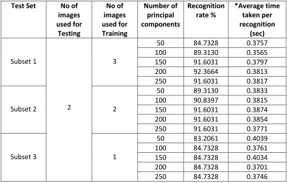
3.10.1.2 Test Result from Procedure 1

In this procedure, the database has been divided into four different subsets. Subset 1

has 6 images which have been used for training and 14 images for testing. Subset 2 has

3 images for training and 17 images for testing, Subset 3 has used only 2 images for

Evaluation and Hardware Realization for a Face Recognition System

Scholarship at UWindsor

Scholarship at UWindsor

Evaluation and Hardware Realization for a Face Recognition

Evaluation and Hardware Realization for a Face Recognition

System

System

Co-Authorship Declaration

Abstract

Acknowledgements

Table of Contents

List of Tables

List of Figures

List of Acronyms

Chapter 1: Introduction

1.1 Why use face recognition software?

1.2 Challenges

1.3 Motivation

1.4 Objective

1.5 Scope

1.6 Organization

Chapter 2: Literature Review

2.1 General Workflow

2.2 Embedded face recognition system

Chapter 3: Software and Algorithm

3.1 Introduction

3.2 A short description on face recognition

3.3 Face Detection

3.4 Facial Alignment

3.5 Feature extraction using Local Binary Pattern (LBP)

3.6 Principal Component Analysis (PCA)

3.7 Processing the Images with LBP and PCA

3.8 Sparse Face Recognition

3.9 Designing the training set

3.10 Results