AN APPROACH OF TRAFFIC FLOW PREDICTION USING ARIMA MODEL WITH FUZZY WAVELET TRANSFORM

University of Windsor University of Windsor

Scholarship at UWindsor

Scholarship at UWindsor

Electronic Theses and Dissertations Theses, Dissertations, and Major Papers

12-20-2018

AN APPROACH OF TRAFFIC FLOW PREDICTION USING ARIMA

AN APPROACH OF TRAFFIC FLOW PREDICTION USING ARIMA

MODEL WITH FUZZY WAVELET TRANSFORM

MODEL WITH FUZZY WAVELET TRANSFORM

Sukruti Vaghasia University of Windsor

Follow this and additional works at: https://scholar.uwindsor.ca/etd

Recommended Citation Recommended Citation

Vaghasia, Sukruti, "AN APPROACH OF TRAFFIC FLOW PREDICTION USING ARIMA MODEL WITH FUZZY WAVELET TRANSFORM" (2018). Electronic Theses and Dissertations. 7608.

https://scholar.uwindsor.ca/etd/7608

This online database contains the full-text of PhD dissertations and Masters’ theses of University of Windsor students from 1954 forward. These documents are made available for personal study and research purposes only, in accordance with the Canadian Copyright Act and the Creative Commons license—CC BY-NC-ND (Attribution, Non-Commercial, No Derivative Works). Under this license, works must always be attributed to the copyright holder (original author), cannot be used for any commercial purposes, and may not be altered. Any other use would require the permission of the copyright holder. Students may inquire about withdrawing their dissertation and/or thesis from this database. For additional inquiries, please contact the repository administrator via email

AN APPROACH OF TRAFFIC

FLOW PREDICTION USING

ARIMA MODEL WITH FUZZY

WAVELET TRANSFORM

BY:

SUKRUTI VAGHASIA

A Thesis

Submitted to the Faculty of Graduate Studies

through the School of Computer Science in

Partial Fulfillment of the Requirements for the

Degree of Master of Science at the University of

Windsor

WINDSOR, ONTARIO, CANADA

2018

October 5, 2018

AN

APPROACH

OF

TRAFFIC

FLOW

PREDICTION

USING

ARIMA

MODEL

WITH

FUZZY

WAVELET

TRANSFORM

By

Sukruti Vaghasia

APPROVED BY:

G. Bhandari

Odette School of Business

J. Lu

School of Computer Science

III

Declaration of Originality

I confirm here I am the sole creator of this theory and no piece of this proposition has been distributed or submitted for production.

I approve to the best of my insight, my proposition does not encroach upon anybody's copyright nor damage any restrictive rights and their thoughts, methods, citations, or some other material from crafted by other individuals incorporated into my postulation, circulation or something else, and are entirely recognized as per the standard referencing hone. Moreover, I have included copyrighted material that outperforms the limits of reasonable managing inside the significance of the Canada Copyright Act. I affirm to acquire a composed consent from the copyright owner(s) to incorporate such material(s) in my postulation and have included duplicates of such copyright clearances to my reference section.

IV

Abstract

It is essential for intelligent transportation systems to be capable of producing an accurate forecast of traffic flow in both the short and long terms. However, the counting datasets of traffic volume are non-stationary time series, which are integrally noisy. As a result, the accuracy of traffic prediction carried out on such unrefined data is reduced by the arbitrary components. A prior study shows that Box-Jenkins’ Autoregressive Integrated

V

Acknowledgments

I might want to express my most profound thankfulness to my supervisor Dr. Xiaobu Yuan for furnishing me with an energizing chance to work in an exciting and testing field of research. His vision helped me to become more creative in my reasoning and furthermore inspired me to inquire.

I would like to offer my gratitude to all the advisory group individuals, Dr. Jianguo Lu and Dr. Gokul Bhandari. Much obliged to all of them for their significant remarks and recommendations to my thesis.

VI

Table of Contents

Declaration of Originality ... III Abstract ... IV Acknowledgments... V List of Tables ... IX List of Figures ... X List of Abbreviations/Symbols ... XII

1. Introduction ... 1

2. Related Work ... 3

2.1. Traffic Flow Prediction ... 3

2.1.1. Summary ... 8

2.2. Technical Background ... 11

2.2.1. Fuzzy Logic Control ... 11

Fuzzy Terminology ... 12

a. Fuzzy Sets ... 12

b. Fuzzification and Membership Functions ... 14

c. Fuzzy Rules for inference ... 16

d. Defuzzification ... 17

i. Mean of Maximum (MOM) Method ... 17

ii. Center of Gravity (COG) Method ... 17

2.2.2. Wavelet Transform ... 20

VII

b. Frequency ... 20

c. Mathematical Transformation of the Signal ... 21

I. Fourier Transform ... 21

a) Stationary Signal ... 21

b) Non-stationary Signal ... 22

The drawback of Fourier Transform ... 23

II. Short-Time Fourier Transformation ... 23

The drawback of Short-Time Fourier Transform ... 24

III. Wavelet Transform ... 25

Sharp Variation Points by Wavelet Transform ... 28

2.2.3. ARIMA Model ... 29

a. Model Structure ... 29

b. Model Identification ... 30

3. Proposed Method ... 34

3.1. Motivations ... 34

3.2. A new hybrid approach using the ARIMA model with Fuzzy wavelet transform ... 35

3.2.1. Design of Algorithm ... 38

4. Implementation and Experiments ... 42

4.1. Experiment Data ... 42

4.2. Performance Evaluation measurements ... 43

4.3. Using Proposed Hybrid Model for Traffic Flow Forecast ... 44

4.3.1. Feature Analysis ... 48

IX

List of Tables

TABLE 1:REVIEW OF PREDICTION METHODS ... 3

TABLE 2SUMMARY OF ADVANTAGES AND CHALLENGES OF CLASSICAL,ANN-BASED, AND SVR TIME SERIES PREDICTION METHODS ... 9

TABLE 3PROPERTIES OF ACF,PACF OF AR,MA AND ARMA SERIES ... 32

TABLE 4FUZZY MEMBERSHIP CATEGORIES ... 36

TABLE 5:FEATURE LIST USED IN TRAFFIC ANALYSIS ... 42

TABLE 6:SAMPLE LIST OF ZERO CROSSING POINTS FOR MATCHING DAYS FOR 26TH DECEMBER ... 45

TABLE 7:FORECAST ACCURACY RESULTS FOR 15 MIN DATASET ... 51

TABLE 8:FORECAST ACCURACY RESULTS FOR TRAFFIC COUNT INTERVAL (15-MINUTE DATASET) ... 51

TABLE 9:FORECAST ACCURACY RESULTS FOR TRAFFIC COUNT INTERVAL (1-HOUR DATASET) ... 52

TABLE 10:FORECAST ACCURACY RESULTS FOR LONG-TERM PREDICTION ... 53

X

List of Figures

FIGURE 1:THE TYPICAL FUZZY LOGIC SYSTEM ... 12

FIGURE 2:REPRESENTATIONS OF CLASSICAL AND FUZZY SETS ... 13

FIGURE 3:FUZZY SET OPERATIONS ... 14

FIGURE 4:MEMBERSHIP FUNCTION OF INPUT AND OUTPUT ... 15

FIGURE 5:MATCHING A FUZZY INPUT WITH A FUZZY CONDITION ... 16

FIGURE 6:GRAPHIC REPRESENTATION OF DEFUZZIFICATION TECHNIQUES WITH MOM METHOD ... 17

FIGURE 7:GRAPHIC REPRESENTATION OF DEFUZZIFICATION TECHNIQUES WITH THE COG METHOD ... 18

FIGURE 8:AN ILLUSTRATION OF FUZZY OUTPUT CALCULATION ... 19

FIGURE 9:DETERMINATION OF FUZZY OUTPUT BY THE CENTER OF GRAVITY METHOD ... 19

FIGURE 10:50HZ SIGNAL ... 20

FIGURE 11THE FT OF THE 50HZ SIGNAL GIVEN IN FIGURE 10 ... 21

FIGURE 12:STATIONARY SIGNAL ... 22

FIGURE 13:FREQUENCY COMPONENT OF FIGURE 12... 22

FIGURE 14:NON-STATIONARY SIGNAL ... 22

FIGURE 15:FREQUENCY REPRESENTATION OF FIGURE 14 ... 23

FIGURE 16:STFT USING A WINDOW FUNCTION ... 24

FIGURE 17:CWT AND DWT OF THE TIME SIGNAL ... 27

FIGURE 18:A PROCESS OF DECOMPOSITION AND RECONSTRUCTION BY WAVELET TRANSFORMS ... 28

FIGURE 19:ACF AND PACF PLOT ... 31

FIGURE 20:ACF AND PACF PLOT AFTER MA(7) ... 32

FIGURE 21:TRAFFIC COUNT COMPARISON OF REGULAR DAYS AGAINST SPECIAL EVENT DAY ... 36

FIGURE 22:TREND IN TIME SERIES ... 37

FIGURE 23:PROPOSED HYBRID ALGORITHM ... 38

FIGURE 24:ORIGINAL TIME SERIES FROM 24TH_{DECEMBER TO 30}TH_{DECEMBER ... 44}

XI

FIGURE 26:DWT OF KNOWN DATA FOR 26TH_{DECEMBER ... 45}

FIGURE 27:THE FIRST PREDICTION OF 26TH DECEMBER ... 47

FIGURE 28:THE SECOND PREDICTION OF 26TH DECEMBER ... 47

FIGURE 29:THE THIRD PREDICTION OF 26TH DECEMBER ... 48

FIGURE 30:TIME SERIES FOR JANUARY 2017 ... 49

FIGURE 31:FOG AS A FEATURE ... 50

XII

List of Abbreviations/Symbols

AR Auto Regression

MA Moving Average

ARIMA Autoregressive Integrated Moving Average ACF Autocorrelation function

PACF Partial Autocorrelation AIC Bayesian information criterion BIC Akaike information criterion ITS Intelligent Transportation System ANN Artificial Neural Network

NN Neural Network

SVM Support Vector Machine

ES Exponential Smoothing

MF Membership Function

DOM Degree of Membership

FT Fourier Transform

WT Wavelet Transform

STFT Short-Time Fourier Transform CWT Continuous Wavelet Transform DWT Discrete Wavelet Transform

SVP Sharp Variation Point

1

1.

Introduction

Urbanization has revolutionized our lives in many aspects. People prefer to live in metropolitan cities rather than countryside. A higher standard of living facilitates us with an individual vehicle instead of using public transportation. It becomes a prominent cause of more vehicles appearing on the road. This problem further leads to other numerous issues such as delay in travel time, increasing traffic jams and accidents, consumption of more fuel, waste of natural resources, etc. Thus, forecasting of traffic is a significant solution for traffic congestion. Advancement in development of traffic sensors, GPS and location detectors can improve the performance of traffic prediction frameworks and the exactness of forecast techniques. Traffic forecast accuracy improves the performance of various components of transportation systems such as corridor management, transit signal priority control and traveler information system [1]. In recent years, traffic forecast has been viewed as a critical segment in the Intelligent Transportation System (ITS). The primary goal of ITS is to add all significant transportation measures to different modes of transport and traffic management and enable users to be better informed and make safer, more coordinated, and 'smarter' use of transport networks [2]. ITS involve information gathering, preparing, and investigating for a specific end goal to guarantee a compelling decision-making tool [3].

2 In the proposed research, a fuzzy method is a crucial part to carry out data categorization as traffic is affected by various events such as a day of week, by weather conditions namely rain, fog, snow and temperature. As mentioned above, considering traffic data as time series data, Discrete Wavelet Transform (DWT) is used to correlate linear and non-linear parts of time series data along with de-noising. Subsequently, Autoregressive Integrated Moving Average (ARIMA) is used to analyze and predict the outcomes of DWT. In the representation of various time series, ARIMA models are widely adapted for precise forecasting. ARIMA considers every time series as linear; however, DWT outweighs this problem by identifying linearity and non-linearity of time series data.

3

2.

Related Work

In this section, some of the relevant background about recent work on traffic flow prediction is discussed, and technical knowledge of the ARIMA model, fuzzy logic, and discrete wavelet transform are studied in detail.

2.1.

Traffic Flow Prediction

“In recent decades, some traffic forecast models have been produced to aid traffic administration and control for enhancing transportation proficiency going from route direction and vehicle navigation to signal coordination. The traffic flow prediction problem can be stated as follows. Let 𝑋_𝑖𝑡 denote the observed traffic flow quantity during the 𝑡𝑡ℎ _{time interval at the 𝑖}𝑡ℎ

observation location in a transportation network. Given a sequence {𝑋_𝑖𝑡} of observed traffic flow data, 𝑖 = 1, 2..., m, 𝑡 = 1, 2..., T, the problem is to predict the traffic flow at a time interval (𝑡 + Δ)

for some prediction horizon Δ.” [6].

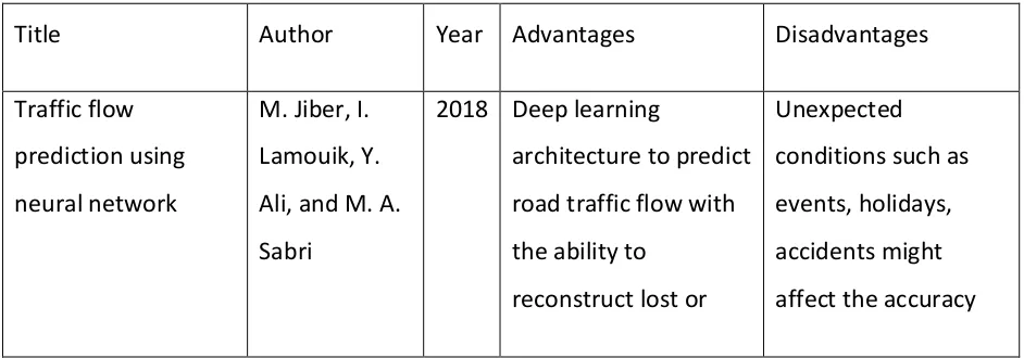
Researchers explored many techniques to forecast traffic volume, Table 1 depicts essential strategies in the territory of traffic flow analysis and traffic flow prediction by posting their favorable circumstances and impediments.

Table 1: Review of prediction methods

Title Author Year Advantages Disadvantages Traffic flow

prediction using neural network

M. Jiber, I. Lamouik, Y. Ali, and M. A. Sabri

2018 Deep learning

architecture to predict road traffic flow with the ability to

reconstruct lost or

4 destroyed data with

the predicted values

Short-Term Traffic

Speed Prediction for an Urban Corridor

H. Zhu, B. Yu 2017 Short-term prediction using support vector machine model with spatial-temporal parameters with higher accuracy

single-step prediction model.

When the traffic

speed is higher than 35 km/h, the

prediction accuracy is reduced

Traffic Flow Prediction using Kalman Filtering Technique

Kumar, S. V. 2017 Uses real time as well as historical (2 days) data for prediction

Nothing has been done for missing values.

Time series Decomposition Model for Traffic Flow Forecasting in Urban Midblock Sections

G. Omkar, S. Vasantha Kumar

2017 Multiplicative decomposition technique is used which requires fewer data compares to ARIMA. Both historical and real-time data are used

5 Improving Traffic

Flow Prediction with Weather

Information in Connected Cars: A Deep Learning Approach A. Koesdwiady, R. Soua, F. Karray

2016 Study of traffic flow prediction with the effect of weather data using deep belief networks.

High usage of memory for the training process.

Traffic Flow

Prediction with Big Data: A Deep Learning Approach

Y. Lv 2015 Examines historical and real-time data to be inputted in a greedy approach which provides

fantastic performance

Takes much time and the data used are produced synthetically Real-time Traffic Flow Predicting Using Augmented Reality

M. Zhang 2016 Produces better accuracy

Doesn’t consider the

chaotic situation, data used to predict is generated

synthetically

Short-term traffic flow prediction using seasonal ARIMA model with limited input data

S. V. Kumar, L. Vanajakshi

2015 Overcome issue of the sound database for ARIMA model by using

past three days’ data.

6 Multi-step

Prediction of Volterra Neural Network for Traffic Flow Based on Chaos Algorithm

L. Yin 2012 Considers both historical and real-time data for long-term prediction

Takes too much time as considers many data.

Early research in traffic predictions used different techniques. For example, in the year 1984, Okutani et al. proposed to apply Kalman filtering [7] with two different models to estimate traffic count. Historical traffic data is more commonly used in some prediction models [8] [9], while others relied on real-time traffic information [10]. For example, Rice et al. used present traffic conditions in Random Walk Forest [11] technique to forecast traffic flow.

7 patterns in traffic data, we can compare related factors of real-time data (forecasting data) with corresponding factors of historical data and only matching a set of data should be considered for further process of prediction [19]. A concept of fuzzy logic as a method of processing data is presented by discussing partial set membership opposite to crisp set membership [20].

Traffic flow prediction methodologies can be ordered into three classes: 1) parametric approach; 2) nonparametric approach, and 3) hybrid approach [15]. The principal strategies of the parametric approach are based on models of autoregressive integrated moving average (ARIMA) [11] [21] [22] and Kalman filtering [23] [24] [25]. Traffic flow has a stochastic and nonlinear nature, but these models predict traffic without considering these characteristics which leads to a substantial error in the prediction.

In the second approach, a nonparametric regression [26] [27] is generally utilized procedure. Chang et al. [9] used a k nearest neighbour nonparametric regression model for short-term traffic prediction. The model claims to achieve better results even with historical time-series data that abruptly changes or widely fluctuates. Liu et al. [28] proposed support vector regression to establish the network traffic prediction model, whereas the global artificial fish swarm algorithm (GAFSA) was used to optimize the model’s parameters. Artificial neural networks (ANNs) were proposed to predict traffic flow [6] [29]. “However, the problem of local minima still exists in ANNs appropriate procedures. What's more, ANNs, most of the time, use one concealed layer. Simulations have exhibited that one hidden layer would not be adequate to depict the convoluted association between the data sources and yields of the forecast model.” [15].

8 linearity and nonlinearity is taken from [31], founded by Zhang, who pointed out that time series data contains both linear and nonlinear patterns. The same approach is taken in [32] which is discussing usage of the piecewise method ARIMA model and the SVM model to predict short-term traffic flow prediction. Tang at el. constructed a fuzzy neural network to forecast travel speed for multi-step-ahead based on two-minute travel speed data [33]. Liu at el. projected use of Adaptive Fuzzy Neural Network (AFFN) for a lane changing predictor to predict steering angles [34]. An approach to tactically utilize the unique strengths of DWT, ARIMA, and ANN to improve the forecasting accuracy is mentioned in [35]. The use of DWT and Fuzzy logic to improve the accuracy of traffic flow prediction on hourly data is shown in [4]. More and more research is being conducted combining two or more methods to predict traffic flow.

Evidently, Khandelwal et al. [30] suggested that neither ARIMA nor ANN is universally suitable for all types of time series. All real-world time series contain both linear and nonlinear correlation structures among the observations. Zhang [4] has pointed out this important fact and has developed a hybrid approach that applies ARIMA and ANN separately for modelling linear and nonlinear components of a time series [35]. Moreover, Adhikari et al. [35] indicated a new hybrid approach which has used DWT to convert the time series in the linear and non-linear component. Based on this approach the proposed method will use the advantage of converting time-series data into linear time series data. Further, it will be used in final forecasting model ARIMA to predict the result.

2.1.1.

Summary

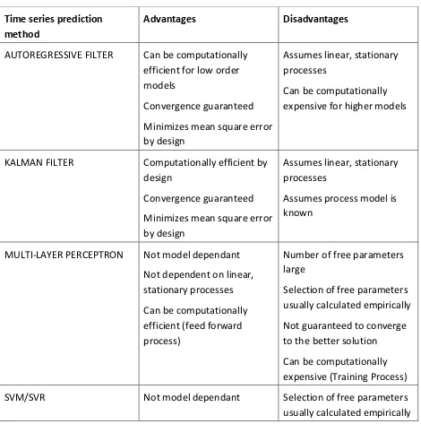
9 predict stochastic nature of traffic series data. There has been no investigation that tries to link the count of traffic data with information from other sources, such as season, weather, the impact of events (traffic accident, planned or unplanned road construction) and time of day and the day of the week. Table 2 [37] lists the pros and cons of available methods used in time series prediction.

Table 2 Summary of advantages and challenges of classical, ANN-based, and SVR time series prediction methods

Time series prediction method

Advantages Disadvantages

AUTOREGRESSIVE FILTER Can be computationally efficient for low order models

Convergence guaranteed Minimizes mean square error by design

Assumes linear, stationary processes

Can be computationally expensive for higher models

KALMAN FILTER Computationally efficient by design

Convergence guaranteed Minimizes mean square error by design

Assumes linear, stationary processes

Assumes process model is known

MULTI-LAYER PERCEPTRON Not model dependant Not dependent on linear, stationary processes Can be computationally efficient (feed forward process)

Number of free parameters large

10 Not dependent on linear,

stationary processes

Guaranteed to convergence to optimal solution

A small number of free parameters

Can be computationally efficient

Can be computationally expensive (Training Process)

Researchers working on traffic prediction have used many advanced algorithms and improved accuracy in forecasting of traffic data. As traffic data is a time series, several outside factors are also responsible for final prediction of result which encourages to introduce Fuzzy Logic. No such prediction model has ever focused on removing noise from data to improve the accuracy of traffic flow prediction and DWT isthe solution. Also, ARIMA is the most widely used forecasting model until now, but its nature of treating every data input as linear can add some error in final prediction of results while using on time series data. DWT is a more suitable method to denoise the time series data and partition into linear and nonlinear. Combination of Fuzzy Logic, DWT and ARIMA will help to achieve higher accuracy model for prediction.

11

2.2.

Technical Background

2.2.1.

Fuzzy Logic Control

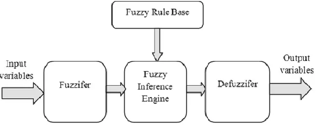
In 1956, Professor L. A. Zadeh, University of California at Berkeley, provided the use of fuzzy logic [19]. Fuzzy thoughts and fuzzy logic even exist in our daily life. A classic example to understand fuzzy logic is the answer to a question as "How satisfied are you with their product or service”? The most likely reply would be 'Not very satisfied' or 'Very satisfied', which are likewise fuzzy or vague answers. Such types of questions can be answered easily by a human, but for a computer, these obscure or vague replies cannot be made easily. The only reply expected from computers is either '0' or '1' for 'HIGH' or 'LOW'. Such outputs are known as crisp or classic output. The fuzzy framework can be viewed as a choice to overcome this issue in the realm of Computer. “To implement a fuzzy logic technique to a real application requires the following three steps:

1. Fuzzification – convert classical data or crisp data into fuzzy data or Membership Functions (MFs)

2. Fuzzy Inference Process – combine membership functions with the control rules to derive the fuzzy output

12

Figure 1: The typical fuzzy logic system1

Fuzzy Terminology

a.

Fuzzy Sets

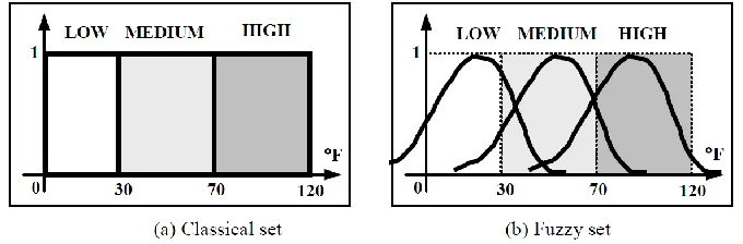
Fuzzy sets are a subset of a classic or crisp set. Difference between standard set and fuzzy sets is the boundary of separating the sets. In classical sets, we have a sharp boundary which means a member belongs to the set or not at all whereas in the fuzzy set we have a smooth boundary with members having a certain membership degree. An example [38] is used here for a better explanation. “If the temperature is defined as a crisp high, its range must be between 80 °F and higher, and it has nothing to do with 70 °F or even 60 °F. However, the fuzzy set will take care of a much broader range for this high temperature. Compared with a classical set, a fuzzy set allows members to have a smooth boundary. In other words, a fuzzy set allows a member to belong to a set to some partial degree. For instance, still using the temperature as an example,

1

13 the temperature can be divided into three categories: LOW (0 ~30 °F), MEDIUM (30 ~ 70 °F) and HIGH (70 ~ 120 °F) from the point of view of the classical set” [38], which is shown in Figure 1.

Figure 2: Representations of classical and fuzzy sets

Any temperature value in the classical set can be classified only in specific subset either in LOW, MEDIUM or HIGH. For instance, temperature value 45 °F is MEDIUM for the classical set. On the other hand, in a fuzzy set, this temperature value falls under LOW with some degree of membership (approximately 0.5 degrees). At the same time, it falls under MEDIUM with around 0.7 degrees of membership. A fuzzy set allows a member to have a partial degree of membership and this partial degree membership can be mapped into a function or a universe of membership values [38].

𝜇_𝐴(𝑥) ∈ [0,1] (𝐴 = (𝑥, 𝜇_𝐴(𝑥)| 𝑥 ∈ 𝑋)) (1)

A fuzzy subset 𝐴 with an element 𝑥 has a membership function of 𝜇𝐴(𝑥) [38]. When 𝑋 is

finite mapping can be represented as in equation (2)

𝐴 = 𝜇𝐴(𝑥1) 𝑥1

+ 𝜇𝐴(𝑥2) 𝑥2

+ . . . . = ∑𝜇𝐴(𝑥𝑖) 𝑥𝑖 𝑖

(2)

When X is continuing the fuzzy set can be defined as in equation (3) 𝐴 = ∫𝜇𝐴(𝑥)

𝑥

14

Figure 3: Fuzzy set operations

Fuzzy set operations are like classical set operations where the union is selecting the maximum of a member from the members and intersect is selecting the minimum member from the sets.

𝑈𝑛𝑖𝑜𝑛: 𝜇𝐴(𝑥) ∪ 𝜇𝑏(𝑥) = max (𝜇𝐴(𝑥), 𝜇𝐵(𝑥))

𝐼𝑛𝑡𝑒𝑟𝑠𝑒𝑐𝑡: 𝜇_𝐴(𝑥) ∩ 𝜇𝑏(𝑥) = min (𝜇𝐴(𝑥), 𝜇𝐵(𝑥))

𝐶𝑜𝑚𝑝𝑙𝑒𝑚𝑒𝑛𝑡: 𝐴𝐶 _{= 𝐹 \ 𝐴}

b.

Fuzzification and Membership Functions

15

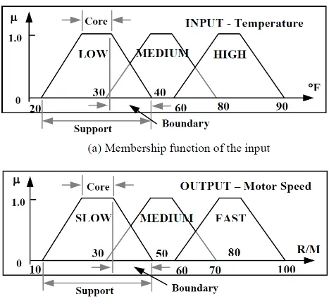
Figure 4: Membership function of input and output

“Continuing the temperature example, we divide the range of temperature as follow Low temperature: 20 °F ~ 40 °F, 30 °F is center

16 To understand more clearly, Figure 4 [38] shows the membership function of these temperatures. For instance, 35 °F will belong to LOW and MEDIUM to 0.5 degrees.” [38]. After defining fuzzy membership functions for input and output the next step is to build a fuzzy rule set. Some terminologies displayed in Figure 4 are as follow. The term “Support” can be explained same as a classical set. For example, support for LOW is a set of elements whose degree in membership LOW is greater than 0. The term “Core” is a set of elements whose degree of membership is equal to one which can be compared to a crisp set. The term “Boundary” is a set

whose degree of membership between 0 and 1.

c.

Fuzzy Rules for inference

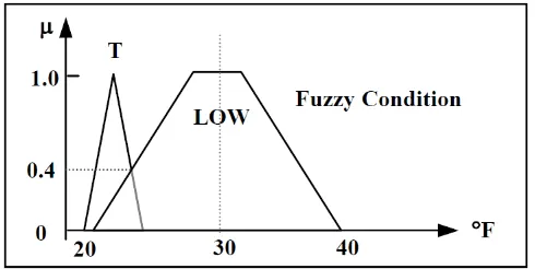
The fuzzy rules are general IF-THEN statements described by some expert or knowledgeable human being of the actual applications. A set of IF-THEN statements describing how the linguistic variable maps to a fuzzy set are introduced to derive conclusions. The antecedent of an IF-THEN statement is an elastic condition to derive the knowledge, whose following part is linguistic output. The inference engine of a fuzzy inference system uses this rule set to calculate the value degree of membership. Figure 5[38] illustrates how the input part or if part of the rule is matched with the defined rules. Here, fuzzy condition LOW and a fuzzy input’s

degree of membership result in membership of 0.4.

17

d.

Defuzzification

The process of defuzzification in a fuzzy system is responsible for converting the fuzzy output to crisp value for real application to use. Remember, the fuzzy conclusion or output is still a linguistic variable, and this linguistic variable needs to be converted to the crisp variable via the defuzzification process [38]. In [38] two defuzzification techniques are discussed which are as mentioned below.

i. Mean of Maximum (MOM) Method

This method calculates the average of output with the highest degree. For example, for the linguistic output, ‘the heater machine is rotated fast’ graphical representation is shown in Figure 6[38]. A shortcoming of the MOM method is that it does not consider the entire shape of the output membership function, and it only takes care of the points that have the highest degrees in that function [38].

Figure 6: Graphic representation of defuzzification techniques with MOM method

ii. Center of Gravity (COG) Method

The most known and used method in the defuzzification process is COG. The weighted average of the membership function or the center of the gravity of the area bounded by the membership function curve is computed to be the crispiest value of the fuzzy quantity [38]. For example, A graphic representation of COG method for the conclusion: ‘the heater motor x is

18

Figure 7: Graphic representation of defuzzification techniques with the COG method

An example of defuzzification with four fuzzy logic rules is described in Figure 8[38]. The first column indicates the value of membership for temperature. The temperature value (𝑇) of 35 °F intersect at 0.6, 0.8, 0.5 and 0.8 for LOW, MEDIUM, LOW and MEDIUM respectively. Likewise, the second column in Figure 8 shows that a temperature change rate (∆𝑇) of 1 °F per hour has the membership functions of 1.0, 0.4, 0.4 and 1.0 [38]. Based on equation (4) the calculation to get the result is min (0.6, 1.0), min (0.8, 0.4), min (0.5, 0.4) and min (0.8, 1.0), which results as 0.6, 0.4, 0.4 and 0.8, respectively [38].

After having fuzzy output from all the four defined rules the next step is to get the crisp or classical value by performing defuzzification using one of the methods defined above. For this study center of gravity is used as COG is a more reliable method than MOM.

Thus, for a temperature of 35 °F and a change rate of temperature 1 °F per hour, the fuzzy output element y for this input pair is 600 R/M [38].

𝑦 = 0.6 × 800 + 0.4 × 300 + 0.4 × 800 + 0.8 × 500

0.6 + 0.4 + 0.4 + 0.8 = 600 R/M

19

Figure 8: An illustration of fuzzy output calculation

Figure 9[38] shows the graphical presentation of fuzzy output to crisp output calculated using COG with the help of four fuzzy rules.

20

2.2.2.

Wavelet Transform

a.

Signal

Any information which can be represented with respect to time can be denoted as a signal. The signal is usually represented in the time domain for most of the time. The signal in its time domain is not always helpful. There might be some information available in its frequency domain as well. To represent the signal in its frequency domain, we need to transform the signal from its time domain to frequency domain. Representation of signal in its frequency format explains what frequency components exist in that signal.

b.

Frequency

The frequency is something to do with the change in the rate of something [39]. Frequency is categorized into two types, low frequency and high frequency. When the change rate is smooth, it is of low frequency; and when the change rate is high, it is of high frequency. As a general example, the daily publication has a higher frequency than monthly publication. To find the frequency of a signal mathematical transformation is applied to the signal. Figure 10 [39] shows the sine wave of 50Hz. Figure 11 [39] shows the mathematical transformation of the sine wave in Figure 10. In Figure 11 there is only one spike at 50 which means the signal in its time domain is stationary no other frequency exists in this signal.

Figure 10: 50Hz signal

21 situation is existing or not but if the frequency component is also analyzed then the diagnosis can be made quickly.

Figure 11 The FT of the 50 Hz signal given in Figure 10

c.

Mathematical Transformation of the Signal

I.

Fourier Transform

In the world of signal Fourier, the Fourier transform (FT) is the most utilized transformation technique. Fourier Transform (FT) processes the time domain signal to frequency domain signal which can be represented by placing frequency content on x-axis and amplitude on the y-axis. If the FT of a signal in the time domain is taken, the frequency-amplitude representation of that signal is obtained [39].

a) Stationary Signal

22

Figure 12: Stationary signal

Figure 13: Frequency component of figure 12

b) Non-stationary Signal

When the signal has different frequency components irrespective of time, such signal is known as a non-stationary signal.

Figure 14: Non-stationary Signal

23 exist in the signal. From the figure, there is no way to identify where in the time which frequency exists in the signal.

Figure 15: Frequency representation of figure 14

The drawback of Fourier Transform

Figure 13 and Figure 15 are Fourier transform of signals in Figure 12 and Figure 14. By comparing Figure 13 and Figure 15 we can see both signals have the same frequencies, i.e., at 10, 25, 50, and 100 Hz except some ripples in Figure 15. Also, there is no similarity in the time domain signal (Figure 12, Figure 14). Both time domain signals have the same frequency component, but in Figure 12 this frequency content exist all the time whereas for Figure 14 this frequency content exists for some fixed interval of time. As mentioned before FT is responsible for identifying the spectral component of any signal. However, FT is not responsible for keeping information of when in the time these frequency content exists. Hence, when the signal is of type non-stationary, FT is not a suitable transform. FT can be used for non-stationary signals, if we are only interested in what spectral components exist in the signal, but not interested where these occur [39]. However, if this information is needed, i.e., if we want to know what spectral component occurs at what time (interval), then the FT is not the right transform to use [39].

II.

Short-Time Fourier Transformation

24 stationary signal. A window function is used to compute the transformation. The signal is divided into the small segments, and on each segment, the window function is applied.

𝑆𝑇𝐹𝑇_𝑋𝑊(𝑡′_{, 𝑓) = ∫ [𝑥(𝑡) ∙ 𝑊(𝑡 − 𝑡}′_{)] ∙ 𝑒}−𝑗2𝜋𝑓𝑡_𝑑𝑡 𝑡

(5)

Here, 𝑥(𝑡) is an original signal, 𝑊(𝑡) is window function, 𝑓 represents the frequency component of the signal, 𝑡′ _{is window time interval, and t is finite time. For every 𝑡}′ _{and 𝑓 a new}

STFT is computed.

Figure 16: STFT using a window function

Figure 16[39] will make it easy to understand how STFT works. The Gaussian-like functions are window function. The red, blue and green colored area shows the window function at time t1’, t2’, and t3’ respectively and this represent the STFT at three different times [39]. Hence, STFT will give us both time and frequency component at the same time.

The drawback of Short-Time Fourier Transform

25 instantaneously. “STFT provides the time intervals in which certain band of frequencies exists, which is a resolution problem. The window size performs the main role in having the time and frequency resolution problems. The narrow window gives good time resolution and poor frequency resolution where wide window gives good frequency resolution and poor time resolution.” [39]

III.

Wavelet Transform

The wavelet transform is used to identify the time-frequency representation of the signal. Wavelet is a small wave. Wavelets have an oscillatory property which works same as window function in STFT. Although the wavelet transform is the transformation process from the time domain to time-scale domain, these processes are known as signal decomposition because a given signal is decomposed into several other signals with different levels of resolution [40].The signal will be passed through several high pass and low pass filters to separate the high frequency and low frequency from the original time domain signal. This process will remove some portion of the signal whenever passed through filters. For instance, a signal with 500Hz frequency when passed through the filters will separate the signal into two signals one containing 0 to 250Hz frequency components of the signal which can be defined as low frequency while the other part is 250-500Hz frequency components which are of high-frequency components. By taking the either or both frequency component, the process will be continued. This process is known as decomposition of the signal. A wavelet transform can easily handle the resolution problem of FT. The WT gives better time resolution in high frequency while better frequency resolution is achieved in low-frequency components. The wavelet transform was used to adopt a wavelet prototype function, which utilized the basic function 𝜓 𝜖 𝐿2(𝑅) that is stretched and shifted to

capture features that are local in time and local in frequency [35]. The transformation function is known as mother wavelet. There are different mother wavelets available in wavelet transform. Wavelet can be defined as pairs of high pass and low pass filters [35].

26 ∫ 𝜑(𝑡) = 1

∞

−∞

And 𝜓𝑗,𝑘(𝑡) = 2

𝐽

2_𝜑(2𝑗_{𝑡 − 𝑘); 𝑗 = 1,2,3 … 𝐽}

∫ 𝜓(𝑡) = 1

∞

−∞

The 𝜑_𝐽,𝑘 is high pass filter whereas 𝜓_𝑗,𝑘 is low pass filter. Hence function 𝑓(∙) can be defined as

𝑓(𝑡) = ∑ 𝑐_𝐽,𝑘𝜑_𝐽,𝑘(𝑡) +

𝑘∈ℤ

∑ 𝑑_𝐽,𝑘𝜓_𝐽,𝑘(𝑡) +

𝑘∈ℤ

… + ∑ 𝑑_1,𝑘𝜓_1,𝑘(𝑡)

𝑘∈ℤ

(7)

We can define the coefficient of both the wavelet as follow 𝑐𝐽,𝑘= ∫ 𝑓(𝑡)𝜑𝐽,𝑘(𝑡)𝑑𝑡 ∞

−∞ and 𝑑𝑗,𝑘 =

∫_−∞∞ 𝑓(𝑡)𝜓_𝐽,𝑘(𝑡)𝑑𝑡; 𝑗 = 1,2,3, … 𝐽 respectively.

27

Figure 17: CWT and DWT of the time signal

28

Figure 18: A process of decomposition and reconstruction by wavelet transforms

If one is interested in visualization, matching or feature detection, CWT might be more useful. If you are interested in denoising, compression, restoration, DWT is more appropriate [43]. The DWT decomposes the time series into different coefficients that represent the signal at different scales which helps to determine local abrupt and regular trend of time series in different scales [44]. There are several wavelets available such as Haar, Daubechies, Meyer, Symlet, etc. Haar wavelet transform has been applied in this research. It is a simple Daubechies wavelet, which is suitable to detect time-localized information and to increase the performance of the prediction technique [45] [46].

Sharp Variation Points by Wavelet Transform

29 wavelet transform, which is called sharp variation points [48]. The researchers proved that on a particular scale, the number of sharp variation points of the traffic flow shows the characteristic of self-similar [48] [47]. We can obtain that a wavelet function 𝜓(𝑥) equals to the first derivative or the second derivative of the smoothing function 𝜃(𝑥) [49]. When 𝜓(𝑥) is chosen as the second derivative of the smoothing function, the zero-crossing of the discrete dyadic wavelet transform related to the closed-contour signal indicates the position of the sharp variation point [49]. The detail coefficients represent positive and negative values. The multiplication between two consecutive coefficients becomes less than zero then those points will be revealed sharp variation points of the signal [4].

𝑊_𝑞(𝑡, 𝑠) ∙ 𝑊𝑞(𝑡 + 1, 𝑠) < 0 (8)

In equation (8), 𝑊_𝑞 is wavelet transformed signal at time t for scales.

2.2.3.

ARIMA Model

The ARIMA model is discussed in [50] first time. It is the most used and classical model for time series analysis. The ARIMA model is based on the fundamental principle that the future values of a time series can be generated from a linear function of the past observations and white noise terms [30].

a.

Model Structure

ARIMA stands for autoregressive integrated moving average. ARIMA is a combination of 3 parts:

1. AR (Auto-Regressive) 2. I (Integrated)

30 An ARIMA (p, d, q) is represented by three parameters: p, d, and q, where p is the degree of autoregressive, d is the degree of integration, and q is the degree of moving average. The Integrated (I) part in ARIMA subtracts time series with its lagged series to extract trends from the data. Autoregressive (AR) extracts the influence of the previous periods’ values on the

current period. Moving Average (MA) extracts the influence of the previous period’s error terms on the current period’s error.

𝑥𝑡 = ∅𝑥𝑡−1+ 𝜀𝑡 ⟹ 𝐴𝑅(1) (9)

Equation (9) for AR with 1 lag is defined in [35]. Lag is a back shift of actual time series which can be any number of units.

𝑥_𝑡 = ∅₁𝑥_𝑡−1+ ∅₂𝑥_𝑡−2+ ⋯ + ∅_𝑝𝑥_𝑡−𝑝+ 𝜀_𝑡 (10)

Here, 𝜀_𝑡 is Gaussian noise and p is order of series. The formula to calculate moving average is

𝑥_𝑡 = 𝜀_𝑡+ 𝜃₁𝜀_𝑡−1+ 𝜃₂𝜀_𝑡−2+ ⋯ + 𝜃_𝑞𝜀_𝑡−𝑞 (11)

Moving average part depends on the noise part of current values as well as past values; it is working as a low pass filter. The combination of autoregressive (AR), moving average (MA) and integrated(I) is ARIMA model, which can be defined as [35]

∅_𝑝(𝐵)(1 − 𝐵)𝑑_(𝑥

𝑡− 𝜇) = 𝜃𝑞(𝐵)𝜀𝑡 (12)

where B is the shift operator and 𝜇 is mean.

b.

Model Identification

31 ACF plots display the correlation between a series and its lags. In addition to suggesting the order of differencing, ACF plots can help in determining the order of the q in ARIMA(p, d, q) model [51]. “The autocorrelation of a time series Y at lag 1 is the coefficient of correlation between Yt and Yt-1, which is presumably also the correlation between Yt-1 and Yt-2. But if Yt is

correlated with Yt-1, and Yt-1 is equally correlated with Yt-2, then we should also expect to find

correlation between Yt and Yt-2. In fact, the amount of correlation we should expect at lag 2 is

precisely the square of the lag-1 correlation. Thus, the correlation at lag 1 ‘propagates’ to lag 2 and presumably to higher-order lags. The partial autocorrelation at lag 2 is therefore the difference between the actual correlation at lag 2 and the expected correlation due to the propagation of correlation at lag 1” [52]. Partial autocorrelation plots (PACF), as the name suggests, display the correlation between a variable and its lags that is not explained by correlations at all lower-order-lags. PACF plots are useful when determining the order of the p in ARIMA(p, d, q) model [53].

Figure 19: ACF and PACF plot

32

Figure 20: ACF and PACF plot after MA (7)

Table 3 represents the idea of selecting the best-fitted model for the forecast.

Table 3 Properties of ACF, PACF of AR, MA and ARMA series

Model Autocorrelation Partial Autocorrelation

AR(p) Tails off gradually Cuts off after p lags

MA(q) Cuts off after q lags Tails off gradually

ARMA(p,q) Tails off gradually Tails off gradually

In addition to ACF and PACF, more techniques are available like AIC (Akaike information criterion) and BIC (Bayesian information criterion) to measure the degree for ARIMA parameters and find the best optimum model.

33 formula for AIC, which provides insight into its relationship to the optimized loglikelihood and its penalty for complexity, is” [54]:

𝐴𝐼𝐶 = −2(𝑙𝑜𝑔𝐿) + 2(𝑛𝑢𝑚𝑏𝑒𝑟 𝑜𝑓 𝑝𝑎𝑟𝑎𝑚𝑒𝑡𝑒𝑟𝑠) (13)

Bayesian Information Criterion: “Like AIC, BIC uses the optimal loglikelihood function value and penalizes for more complex models, i.e., models with additional parameters. The penalty of BIC is a function of the sample size, and so is typically more severe than that of AIC. The formula for BIC is” [54]:

34

3.

Proposed Method

This chapter discusses the characteristics of data for time series analysis, the architecture of the algorithm and steps involved by flowcharts and block diagrams of the proposed hybrid algorithm.

3.1.

Motivations

Before delving into the study of traffic prediction, the findings of the related work discussed in previous chapters gave solid reasons which need to be considered while predicting the time series. These issues mentioned in 2.1.1 must be considered while forecasting the traffic flow. A significant part of the current work focuses on the short-term forecasting which helps to improve the decision-making process of traffic lights or online map system to guide the user to take a less time-consuming road [21]. On the other hand, the long-term traffic prediction is helpful to those who are planning a journey and can anticipate their travel time in advance to reach their destination in time [21].

In the proposed method some of the pitfalls of previous work have been addressed in the following two aspects.

• Model:

Prerequisite of a model which is trustful under all circumstances. The model should be able to work for adjustable time spans. It should be able to handle missing information, capture the changing trend of information and work with stochastic data.

• Accuracy:

35

3.2.

A new hybrid approach using the ARIMA model with Fuzzy wavelet

transform

In time series forecasting, identifying the abnormal behavior of traffic flow from the vast dataset and finding the reason behind irregular traffic pattern can help to identify the changing trend. The reason behind such an abnormal traffic count can be any special events such as accidents, severe weather conditions, roadwork, or vehicle breakdown. We can find such a trend when time series data starts to behave irregular from usual daily traffic patterns.

The characteristic of the traffic flow forecast is hard to capture. From Figure 21, for 25th

July and 26th _{July the flow of traffic is almost similar. For 27}th _{July significant fluctuation from}

36

Figure 21: Traffic count comparison of regular days against special event day

A fuzzy classifier is used to compare real data with stored data to the degree of membership. From the definition of the degree of membership denoted by μ, first the level of preciseness is defined. Three categories of preciseness as described in Table 4 which depends on the value obtained from the degree of membership. As these values range from 0 to 1, the degree of membership can be defined as μ [0,1]. The degree of membership of any historical traffic dataset will be determined based on similarities between real-time dataset and historical dataset [4].

Table 4 Fuzzy membership Categories

37 Based on the number of factors NC (number of data components) this method classifies

dataset as HSD for having 8 similar data out of 11, as MSD for having at least 4 similar data , or as LSD for having at least 3 similar data out of 11 [3]. Here NC can vary based on used dataset and

similarity will be adjusted accordingly. Based on the calculated membership degree, days with the highest membership degree will be used only for the further process of the forecast. If the selected featured dataset is not matching with HSD, the system looks for a matched MSD with minimal discrete distance. And lastly, the system looks for an LSD dataset if there is no MSD with minimal discrete distance exist.

Evidently, Khandelwal et al. [30] suggest that neither ARIMA nor ANN is universally suitable for all types of time series. Almost all real-world time series contains both linear and nonlinear correlation structures among the observations [30].

Figure 22a: From 6:00 am to 10 am Figure 22b: From 2:00 pm to 6 pm

Figure 22: Trend in Time Series

38 and non-linear component. The proposed method will use the advantage of converting time-series data into linear time time-series data. Another advantage of using DWT as discussed in [56] is to apply the transformation to approximation coefficients in each layer. The filter is used to recognize local dependencies in the data, which are subsequently combined to represent more global features until the output of interest is computed in the final layer. These coefficients will be further used in final forecasting model ARIMA to predict the result.

3.2.1.

Design of Algorithm

Figure 23: Proposed Hybrid Algorithm

39 ARIMA model. The one with an optimal (p, d, q) will be used. After getting an optimal linear time series from ARIMA inverse DWT will be applied to construct the predicted traffic time series.

Algorithm 1: ARIMA MODEL WITH FUZZY WAVELET TRANSFORM

INPUT: X = {xt, t = 1,2, … , n}, where xt is a value at discrete time t

OUTPUT: Predicted traffic from t + i as (xt+ i) where i is the forecasting period

1. train_dataset ← 70% of the dataset

2. real_time_dataset ← 30% of dataset

3. CategorizModels ← FuzzySystem(train_dataset)

4. foreach(x in CategorizModels)

4.1. trained_coeffs ← dwt(x, filterlevel, filtertype)

4.2. SVP(trained_coeffs)

5. trained_arima_model ← arima(trained_coeffs)

6. foreach(𝑋𝑡 in real_time_data)

6.1. DOM ← FuzzySystem(𝑋𝑡)

6.2. Model ← CategorizModels(DOM)

6.3. coeffs ← dwt(Model, filterlevel, filtertype)

6.3.1.foreach(𝑋̂𝑡 in Model )

6.3.1.1. distance ← √∑ (𝑋𝑡− 𝑋̂𝑡) 2 𝑇

1 ⁄𝑇

6.3.2. data ←𝐷𝑎𝑦𝑜𝑓𝑀𝑖𝑛𝑖𝑚𝑢𝑚(distance)

6.4. i ← Find distance between two nearest consequent SVPs from data

40 7. Go for next (xt+ i) + 1

8. End

In the 1st _{and 2}nd _{steps, a dataset will be divided into training and testing datasets. Training}

41

Algorithm 2: Fuzzy System

INPUT: train_dataset OUTPUT: CategorizModels

1. Determine the required features as variables of the fuzzy system to partition datasets into HSD, MSD, and LSD

2. Define fuzzy rules to map the variables to one of the categories (HSD, MSD, LSD) 3. Calculate the degree of membership for each rule

4. Divide the dataset into (HSD, MSD, LSD)as per the specified boundary of membership for each partition

42

4.

Implementation and Experiments

4.1.

Experiment Data

There are three datasets used in the experiment of the proposed method. Among them, one is constructed to include all the features listed in Table 5 and the other two consist of only weather data as a feature for analysis purpose. The first data set is taken from Highways England for site M1/4771B (MIDAS site at M1/4771B priority 1 on link 116019002; GPS Ref: 432323;405646; Southbound) [57]. For the same geographical position, the event data is taken from Traffar: UK Current traffic information where all the event related to M1 southbound junction 37 is available. The weather data for the same location is taken from timeanddate.com for nearby city Barnsley, England, United Kingdom. All the data of weather and events are considered as feature data. Table 5 is a list of features considered in the experiment. The time interval is 15 minutes.

Table 5: Feature List used in Traffic analysis

Feature Type Feature Name Feature Number

Weather Snow 1

Wind 2

Humidity 3

Fog 4

Temperature 5

Precipitation 6

Duration 7

Holiday 0 or 1 (0 is holiday, 1 no holiday)

8

Day after holiday 0 or 1 (0 is the day after the holiday, 1 regular)

43 Event Accident or Roadwork or

vehicle breakdowns

10

Geographic Location Highway or Intercity 11 The second dataset provides a minute by minute traffic flow for Junctions 25 to 30 of the M62. Traffic data is recorded via inductive loops by the MIDAS Subsystem (Motorway Incident Detection and Automatic Signalling) for those sites that have been enabled as traffic counting sites [58]. The weather data for nearby city Brighouse HD6 4HG, UK is taken. The third dataset is traffic data provided by Washington State Department of Transportation (WSDOT), USA. WSDOT determines traffic count data from most of the roads in the city road network [4]. This research uses traffic count for the road at Rhododendron, Coupeville on milepost 20:02 point, Eastbound [4].

4.2.

Performance Evaluation measurements

We utilize three performance measures to identify the appropriateness of the proposed method which are the mean relative error (MRE), root-mean-square error (RMSE) and mean absolute percentage error (MAPE) as described in [6]

𝑀𝑆𝐸 = 1

𝑛∑ |𝑓𝑖 − 𝑓̂|𝑖

𝑛

𝑖=1

(15)

𝑀𝐴𝑃𝐸 = 1 𝑛∑

|𝑓_𝑖 − 𝑓̂|_𝑖 𝑓_𝑖

𝑛

𝑖=1

× 100 (16)

𝑅𝑀𝑆𝐸 = [ 1

𝑛∑(|𝑓𝑖 − 𝑓̂|)𝑖 2 𝑛 𝑖=1 ] 1 2 (17)

44

4.3.

Using Proposed Hybrid Model for Traffic Flow Forecast

The dataset of the 15-minute time interval is for almost one year. In Figure 24 the original time series has fluctuation which is an indication of noise. Therefore, after using the discrete wavelet transform, we have eliminated such noise as shown in Figure 25. Also, an analysis can be made from the Figure 25 that a regular recurrence at a particular time is present in the time series. The traffic flow starts to increase from 5 a.m. to 6 a.m. and keep increasing until 10 a.m. in the morning. After 10 a.m. to 4 p.m. almost decreases and then again between 5 p.m. to 6 p.m. increases in traffic can be seen in Figure 25. By identifying such trends, we can quickly build a model that follows them. The trend detection proposed in [50] used zero crossing detection to identify the trend in the time series. In Figure 26, DWT shows the changing trend in the topmost plot. After applying DWT, we can even trace the minor details available in time series. Also notice here that the 2nd _{and 3}rd _{and 4}th _{spikes are higher than other spikes. It is a holiday on 25th and}

Figure 24: Original Time Series from 24th

December to 30th _December

Figure 25: Denoised Time Series from 24th

December to 30th _December

45 discrete wavelet transform to spot such trends and for long-term traffic prediction as described in the previous section.

Figure 26: DWT of known data for 26th _December

As per step 6.1 and 6.2 in the algorithm, all the datasets for similar features will be derived using Fuzzy system rules.

Table 6: Sample list of Zero crossing points for matching days for 26th December

46 Then using the distance calculation formula√∑ (𝑋𝑡− 𝑋̂𝑡)

2 𝑇

1 ⁄𝑇 , where 𝑋𝑡 is prediction

day and 𝑋̂_𝑡 is matching day, a distance of each day with the prediction day will be calculated and stored. Then the data with minimum distance will be retrived which is a list of trained coefficients of matching day. In step 6.3 find the distance between the nearest two zero crossing points of matching day and pass it along with trained coefficients and the calculated optimized model to forecast upto the distance between two crosing points. For an example, Suppose prediction day is 26th _{december as shown in Figure 26 start from the initial time of 12 a.m. for the forecast.}

Based on the distance calculation formula the closest trend that matched for similar duration of day 26th _{December 2017 will be calculated, which is 1}st _{January 2017. Next two sharp variation}

point for the matched day will be retrieved. From Table 6, the first two sharp variation points are 33 and 52 which is from 8 a.m. to 1 p.m. So, the first prediction for 26th _{December can be done}

using 1st _{January’s data from 8 a.m.(t=33) to 1 p.m. (t=52) which is plotted in Figure 27. Then}

repeat the same procedure for the second prediction. The second closest match found for the same day is 14th _{April 2017. The next two sharp variation point from 14}th _{April is 2 p.m. (t=51) to}

5 p.m.(t=70) which is shown in Figure 28. The third closest matching trend found for the duration of 5 p.m.(t=69) to 11 p.m.(t=86) is 29th _{April 2017 and the prediction for that time is depicted in}

47

Figure 27: The first prediction of 26th December

48

Figure 29: The third prediction of 26th December

4.3.1.

Feature Analysis

49

Figure 30: Time series for January 2017

A fascinating perception made here is that the preferred location is busy during weekdays and less busy during weekends. Though for the 1st _{December 2017 Sunday, the traffic seems high}

than other Sundays. The reason behind this rush can be the new year’ day which inspires to select the seasonal holiday as a feature. Traffic rush difference between weekdays and weekend is also an important feature that affects the traffic count. In Figure 21 we compare the regular days against some days where special events like roadwork or accident happened which encourages to include those events in our feature list for traffic count dataset. Figure 31 shows the effect of fog on traffic count. Weather data suggest that on 6th _{and 8}th _{February there was fog in morning}

50

Figure 31: Fog as a feature

4.4.

Experiments and Results

Above feature analysis leads to two types of traffic prediction cases. One is a special day while the other is an average day with no special events.

51 Table 7 shows the proposed algorithm is giving better accuracy compared to other traditional models. As the interval of time series is increasing, the accuracy is decreasing, but the proposed approach outperformed other models for long-term as well as short-term predictions. We can say that our model is more reliable with small interval time series.

Table 7: Forecast Accuracy Results for 15 min dataset

Short-Term Traffic Prediction Long-Term Traffic Prediction 10 Min 20 Min 30 Min 60 Min 2 hours 4 hours 8 hours 16 hours CATA 95.0 94.3 94.0 87.0

CATB 87.3 87.4 87.3 88.6 Slip-road 92.2 91.5 92.1 84.7

Velorra 92.18 92.07

RBFNN 94.79 89.96

Hossain J 95.13 93.86 94.96 80.69

Hybrid ARIMA 99.89 99.45 98.49 97.7 96.25 95.49 95.10 83.49

Case 2: Rainy day, a day when the accident happened and holidays for traffic prediction. The steps of prediction will be the same as discussed in case 1. The only difference between these two cases is that we will add features to a model dataset which will be further used by ARIMA for final predictions.

Table 8: Forecast Accuracy Results for Traffic Count Interval (15-minute dataset)

Hybrid ARIMA ARIMA

MAE MAPE RMSE MAE MAPE RMSE Rainy Day (Fri, Mar

3)

52 Accident (Thus,

July 27)

0.9878688 2.186649 1.307614 15.14474 16.20278 18.1965

Holiday (Tue Dec 26)

0.5264768 1.667271 0.6604433 12.8223 19.3160679 22.241

Table 8 and Table 9 shows that including features data improve the accuracy of prediction. The forecast result of Table 8 for a rainy day, holiday and day after a holiday is 98.48%, 97.82%, and 98.33% MAPE, respectively while for the same days if features are excluded then accuracy measure MAPE drops to 86.69%, 83.80%, and 80.68%. That depicts the external factors directly relate to traffic count.

Table 9: Forecast Accuracy Results for Traffic Count Interval (1-hour dataset)

Hybrid ARIMA ARIMA

MAE MAPE RMSE MAE MAPE RMSE Rainy Day (Thu, Nov

30)

2.839904 2.942747 3.474441 14.97356 17.20757 18.23457

Holiday (Thu Nov 23) 1.797659 1.306445 2.292871 17.30464 18.339838 19.30214 Day after Holiday (Thu

Dec 26)

0.842441 1.211623 2.504301 17.97094 17.315016 19.46874

53

Table 10: Forecast Accuracy Results for Long-Term Prediction

Long-Term Prediction (MAPE)

1st _{prediction 2}nd _{Prediction 3}rd _Prediction

Rainy Day (Thu, Nov 30)

96.02% 95.45% 93.48%

Holiday (Thu Nov 23) 93.56% 92.76% 93.49%

Table 10 represents the results when prediction duration is derived from zero crossing points. The prediction day 30th _{Nov with featured data is used in 1}st _{prediction, the trend from 8}

a.m. to 2 p.m. of day on 8th _{November is closely matching based on distance calculation formula.}

Hence, the first prediction is up to 2 p.m. on that day. The second prediction trend is closely matched with 15th _{November from 2 p.m. to 7 p.m. The last prediction trend is closely following}

the 29th _{November. The average prediction accuracy achieved with this method is 94.98%.}

Figure 32: Comparison with different Forecast Models

60 70 80 90 100

8:14:00 8:44:00 9:14:00 9:44:00 _{10:14:00 10:44:00 11:14:00 11:44:00 12:14:00 12:44:00 13:14:00 13:44:00 14:14:00 14:44:00 15:14:00 15:44:00 16:14:00 16:44:00 17:14:00 17:44:00 18:14:00 18:44:00 19:14:00 19:44:00 20:14:00 20:44:00 21:14:00 21:44:00 22:14:00 22:44:00 23:14:00 23:44:00}

54 The forecasting result in Figure 32 is of short-term results for a single day from different time series prediction models. It can be noticed that the proposed model outperformed among all. The classic ARIMA model has a lowest average accuracy of 82.33%. The Exponential Smoothing model has 88.27% average accuracy. The neural network model has better performance result than any other model with an accuracy of 93.67%. The neural network exhibits similar results as Hybrid ARIMA. However, the proposed model of prediction yields better results with the highest accuracy of 95.49%.

Table 11: Short Term Forecast Accuracy for one day

Prediction Models MAPE (%) ARIMA 82.33 Exponential Smoothing 88.27 Neural Network 93.67

Hybrid ARIMA 95.49

55

5.

Conclusion

As the civilization is developing the problem of traffic on the road is increasing on daily basis. To help people tackle with traffic problems the best option is to know the situation of traffic in advance, so people can manage their work and save their time by adjusting their daily schedule of traveling. In thesis proposal, we presented a time series forecasting based on the combination of Fuzzy logic, wavelet analysis, and ARIMA. We have shown how the fuzzy logic is built to categorize data to provide more accurate data in the prediction model. The results state that if data is classified then better accuracy can be achieved. Usually time series ARIMA forecasting model uses past data with lagged value. Fuzzy logic in this model is used to build the dataset by considering only those past data which are most relevant to the prediction duration. For example, if the day is Monday and season is winter, then only those data with higher frequency matching will be selected which helps to get the more fitted model in ARIMA process. The multi-scaling property of the DWT enhances the prediction of non-linear and denoised traffic time series, and finally, ARIMA is used as a prediction model for long-term as well as short-term traffic prediction. For long-term traffic prediction, we have used sharp variation points to examine the detail level of traffic fluctuation to forecast for a certain period.

• Model:

The model builds in this thesis using the hybrid approach is trustful under all circumstances. The model can work for adjustable time spans, short-term as well as long-term. The use of DWT handles the missing information, capture the changing trend of information and work with stochastic data. The ARIMA being classical forecasting method along with fuzzy and DWT shows the more improved results.

• Accuracy:

56 classification can be even more accurate. This helps to build the model for more accurate prediction.

57

References

[1] L. LI, W.-H. Lin and H. Liu, "Type-2 Fuzzy Logic Approach for Short-term Traffic

Forecasting," in IEE Proceedings-Intelligent Transport Systems, vol. 153, IET, 2006, pp. 33--40.

[2] "Intelligent Transportation Systems," People.ece.umn.edu, [Online]. Available: http://people.ece.umn.edu/~mhong/Project_ITS.html. [Accessed 17 09 2018].

[3] M. Jiber, I. Lamouik, Y. Ali and A. Sabri, "Traffic flow prediction using neural network," in

Intelligent Systems and Computer Vision (ISCV), 2018 International Conference on, IEEE, 2018, pp. 1--4.

[4] J. Hossain, "A Hybrid Approach of Traffic Flow Prediction Using Wavelet Transform and Fuzzy Logic," University of Windsor, Windsor, 2017.

[5] T. J. Ross, Fuzzy logic with engineering applications, John Wiley & Sons, 2009.

[6] Y. Lv, Y. Duan, W. Kang, Z. Li, F.-Y. Wang and others, "Traffic flow prediction with big data: A deep learning approach," IEEE Trans. Intelligent Transportation Systems, vol. 16, no. 2, pp. 865--873, 2015.

[7] I. Okutani and Y. . J. Stephanedes, "Dynamic prediction of traffic volume through Kalman filtering theory," Transportation Research Part B: Methodological, vol. 18, no. 1, pp. 1--11, 1984.

[8] M. o. T. Ontario, Advanced Traffic Management System, 2007.