Dynamic Modeling and Control of Distributed Generation System Driven by Solid-State Transformers: A Nonlinear Dynamical Approach.

(1)

ABSTRACT

KHAN, MD TANVIR ARAFAT. Dynamic Modeling and Control of Distributed Generation System Driven by Solid-State Transformers: A Nonlinear Dynamical Approach. (Under the direction of Drs. Iqbal Husain and Aranya Chakrabortty.)

With advances in power electronic components and their controls, the penetration of renewable energy resources into the traditional power grid is steadily increasing. Higher penetration of the renewable sources causes power quality and stability problems such as voltage rise, frequency fluctuation, and subsequent impacts on the customer side. To address the penetration issues and facilitate the integration of renewable energy, the Future Renewable Electric Energy Delivery and Management (FREEDM) system has developed a power electronics based solid-state transformer (SST) which serves as an energy router for the power distribution system. SST interfaces distributed generation, storage and local loads on the low voltage side with the medium voltage node of the distribution grid. In this research, a physics based comprehensive dynamic model of FREEDM system is developed to analyze the feasibility based on system equilibrium which is one of the necessary conditions for stable operation of any power distribution system. State-space modeling of the SST along with the renewable generation sources and storage components has been adopted as the means of studying the feasible operating points and analyzing the dynamic behavior of the FREEDM system. The actual model of the single-SST system is a highly complex one with more than hundred state variables. Model reduction techniques are applied that leads to a 70th order state-space average model, which is suitable for AC and DC energy cell system sizing, stability analysis, and controller design.

(2)

and simulated by maintaining the node voltage or input current constant with a step change in any SST in the neighborhood. Energy storage and photovoltaic (PV) ‘plug-and-play’ units have important roles in the power sharing methods in the microgrids. Energy storage control for the microgrid has been developed considering instantaneous change from renewable generation or load demand; the storage controller can also assist in power sharing methods respecting the feasibility bounds with known system parameters and generation capacity of renewables.

(3)

(4)

Dynamic Modeling and Control of Distributed Generation System Driven by Solid-State Transformers: A Nonlinear Dynamical Approach

by

Md Tanvir Arafat Khan

A dissertation submitted to the Graduate Faculty of North Carolina State University

in partial fulfillment of the requirements for the degree of

Doctor of Philosophy

Electrical Engineering

Raleigh, North Carolina 2018

APPROVED BY:

_______________________________ _______________________________

Dr. Iqbal Husain Dr. Aranya Chakrabortty Committee Co-Chair Committee Co-Chair

_______________________________ _______________________________

(5)

DEDICATION

(6)

BIOGRAPHY

Md Tanvir Arafat Khan received his B.Sc. degree in Electrical and Electronic Engineering (EEE) from Bangladesh University of Engineering and Technology (BUET), Dhaka, Bangladesh, in 2011. He received his M.Sc. and Ph.D. degree from the department of Electrical and Computer Engineering at North Carolina State University, Raleigh, NC in 2014 and 2018, respectively.

(7)

ACKNOWLEDGMENTS

I express my deepest gratitude to my advisors Drs. Iqbal Husain and Aranya Chakrabortty for their sincere guidance and advice to pursue my doctoral study. Dr. Husain is a passionate researcher and mentor from whom I learnt to conduct the research in a way that leads to a meaningful contribution. Dr. Chakrabortty is a dedicated adviser whose continuous guidance and assistance were essential to the completion of this research. I would also like to thank my dissertation committee members, Dr. Wensong Yu and Dr. Andre Mazzoleni for their valuable suggestions and support. I also thank Dr. Rafael Cisneros Montoya for his guidance during the last year of my PhD.

I would also like to thank all the faculty, students and staffs working at the NSF FREEDM Systems center for providing tremendous support and encouragement since I joined here in 2013. A special thanks goes to Karen Autry for her endless support to make my life easier from the very first day in the center. I would also like to thank Alireza Afiat Milani for being a great friend and partner in our microgrid system modeling and control research. I would like to thank Ritwik Chattopadhyay and Gregory Norris for their every suggestion and help in the experimental work.

(8)

TABLE OF CONTENTS

LIST OF TABLES ... viii

LIST OF FIGURES ... ix

Chapter 1: Introduction ... 1

1.1 Research Background ... 2

1.2 Research Motivation ... 6

1.3 Contribution ... 8

1.4 Dissertation Outline... 9

Chapter 2: Dynamic Modeling and Feasibility Analysis of a Solid-state Transformer Based Power Distribution System ... 12

2.1 Introduction ... 13

2.2 Detailed Modeling of FREEDM System ... 14

2.2.1 SST – Rectifier Model and Controllers ... 15

2.2.2 SST – DAB Model and Controllers ... 17

2.2.3 SST – Inverter Model and Controllers ... 18

2.2.4 DRER Model and Controllers ... 21

2.2.5 DESD Model and Controllers ... 23

2.3 Case Studies with the Developed Average Model ... 26

2.4 Feasibility and Stability Surface Plots Based on Rectifier Model ... 31

2.6 Conclusions ... 34

Chapter 3: Power Sharing Methods in a Multiple SST Based System ... 35

3.2 Single SST Feasibility Constraints and Expansion to Multi-SST Case ... 38

3.2.1 Feasibility Analysis of Rectifier ... 38

3.2.2 Multi-SST Circle Condition to Manintain Feasibility ... 40

3.3 Proposed Power Sharing Methods to Maintain Feasibility ... 42

3.3.1 Method 1: Power Sharing with Constant Input Current ... 44

3.3.2 Method 2: Power Sharing with Constant Node Voltage ... 47

3.4 Case Studies with Different Conditions to Verify the Proposed Methods ... 48

(9)

Chapter 4: Microgrid Storage Control in FREEDM System ... 62

4.2 Energy Storage in FREEDM System ... 66

4.3 Input-output Controller for the Energy Storage ... 71

4.3.1 Controller Derivation for Energy Storage ... 73

4.3.2 Stability of Energy Storage Controller with Multiple SSTs ... 75

4.4 Storage Controller for Power Sharing Methods ... 81

4.4.1 Storage Controller Implementation for Power Sharing Method 1 ... 83

4.4.2 Storage Controller Implementation for Power Sharing Method 2 ... 85

4.5 Validation of the Storage Controller ... 85

Chapter 5: System Simulation in IEEE 34 Bus Distribution Network ... 94

5.2 IEEE 34 Bus System Model and Description ... 95

5.3 Feasibility Analysis in IEEE 34 bus ... 96

5.4 Implementation of Power Sharing Methods in IEEE 34 Bus... 103

5.4.1 Storage Controller with Method 1 ... 103

5.4.2 Storage Controller with Method 2 ... 114

Chapter 6: ‘Plug-and-Play’ Installation for DC-AC Microgrids with Expedited Permitting Device ... 126

6.2 Current PV System Permitting Requirements ... 130

6.3 ‘Plug-and-Play’ PV Electrical System ... 131

6.4 Multi-port Building Block (MPBB) ... 135

6.5 Photovoltaic Utility Interface (PUI) ... 137

(10)

6.7 Prototype and Experimental Results ... 144

6.8 Cost Analysis of the System... 151

Chapter 7: Summary and Future Work ... 154

7.1 Summary ... 155

7.2 Future Work ... 156

(11)

LIST OF TABLES

Table 2.1 FREEDM system parameter list ...19

Table 3.1 Simulation data of the nine SST system validation ...49

Table 6.1 PUI ‘plug-and-play’ software functions ...142

Table 6.2 Byte data examples for PnP communications ...143

Table 6.3 Communications protocol example ...143

(12)

LIST OF FIGURES

Figure 1.1 Average annual growth rates of renewable energy ...2

Figure 2.1 One node FREEDM system model ...17

Figure 2.2 Solid-state transformer circuit model ...18

Figure 2.3 PV DRER, boost converter and rectifier for PV AC interface ...22

Figure 2.4 PV DRER and boost converter for PV DC interface ...22

Figure 2.5 DESD and rectifier circuit for AC DESD average model ...25

Figure 2.6 DESD and buck-Boost circuit for DC DESD average model ...25

Figure 2.7 Case studies with 70th order average model ...28

Figure 2.8 Case study with regenerative mode of operation ...29

Figure 2.9 Case study with input voltage variation ...29

Figure 2.10 Case study with active power variation ...30

Figure 2.11 Case study with parameter variation ...30

Figure 2.12 Expansion of feasibility region by reducing rectifier resistance ...32

Figure 2.13 Feasibility and stability circle diagram ...33

Figure 2.14 Expansion of stability region by retuning the controller gains ...33

Figure 3.1 FREEDM system functional diagram ...39

Figure 3.2 Circuit diagram of a solid-state transformer ...39

Figure 3.3 Simplified tree configuration with multi-SST ...41

Figure 3.4 Different cases with change in power ...43

Figure 3.5 Radial network of FREEM system ...44

Figure 3.6 Net power of each SST by applying method one ...51

(13)

Figure 3.8 Input current of each SST by applying method one ...53

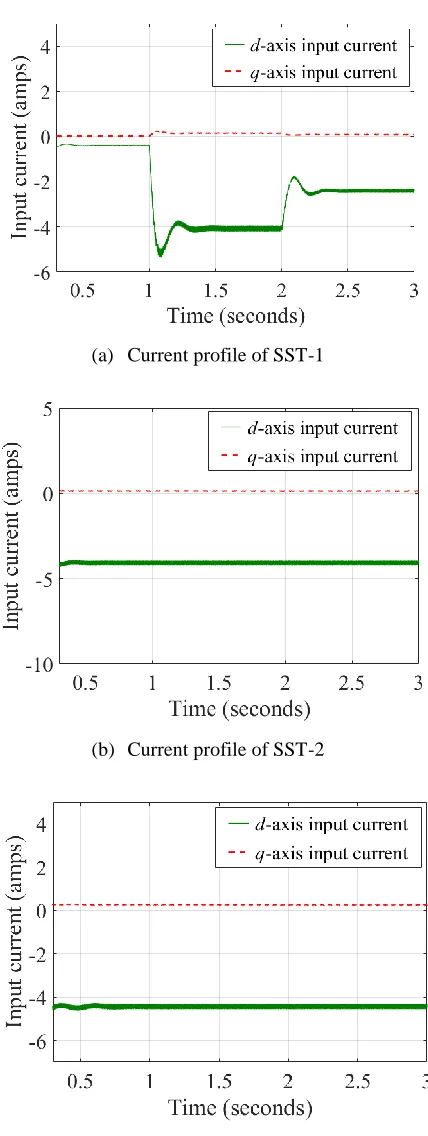
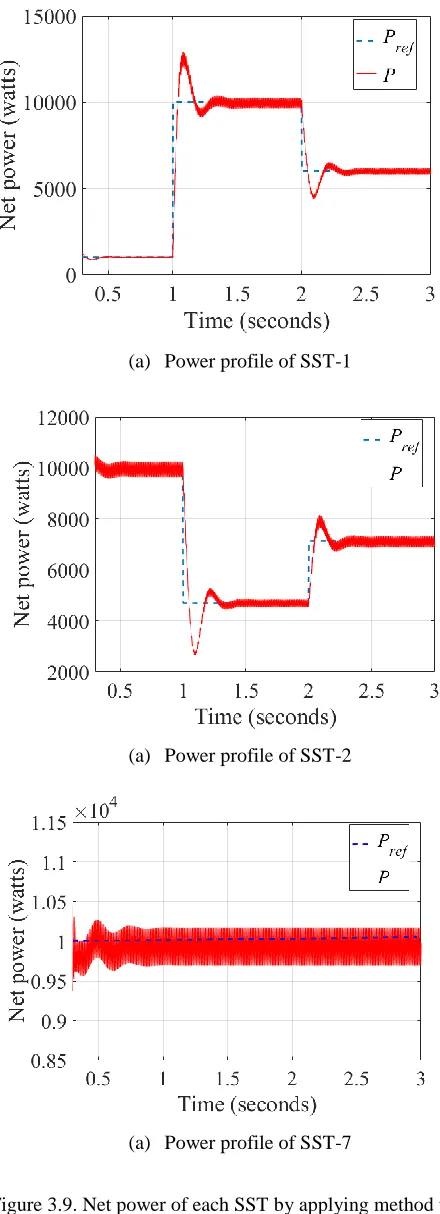
Figure 3.9 Net power of each SST by applying method two ...54

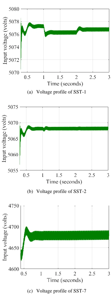
Figure 3.10 Input voltage of each SST by applying method two ...55

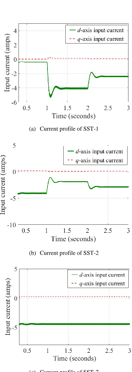
Figure 3.11 Input current of each SST by applying method two ...56

Figure 3.12 Control architecture of FREEDM system ...58

Figure 3.13 Control interaction between IEM and IPM ...59

Figure 3.14 Timescale separation of the controller in FREEDM system ...60

Figure 4.1 Power change scenario in FREEDM system ...67

Figure 4.2 SST configuration for energy storage controller ...69

Figure 4.3 DESD interface circuit with DC-DC converter ...71

Figure 4.4 Simplified structure of the DC microgrid ...73

Figure 4.5 Controller implementation diagram ...76

Figure 4.6 Plot for the stability functions ...77

Figure 4.7 Load change cases in FREEDM system ...82

Figure 4.8 Power sharing implementation in cyber-physical layer ...84

Figure 4.9 Storage profile for SST 1 to SST 3 ...86

Figure 4.12 DAB output voltage profile for SST 1 to SST 3 ...88

Figure 4.15 Rectifier output voltage profile for SST 1 to SST 3 ...90

(14)

Figure 4.17 Rectifier output voltage profile for SST 7 to SST 9 ...91

Figure 5.1 PSCAD circuit model for the IEEE 34 bus with SSTs ...96

Figure 5.2 PSCAD schematic model for the IEEE 34 bus with SSTs ...97

Figure 5.3 Screenshot of the LSSS model in PSCAD ...98

Figure 5.4 SST input voltage (d-axis) in IEEE 34 bus simulation ...100

Figure 5.5 Rectifier output voltage in IEEE 34 bus simulation ...101

Figure 5.6 Failure analysis for distant SST in IEEE 34 bus ...102

Figure 5.7 Storage response of SST 1 to 3 ...104

Figure 5.10 Power profile of SST 1 to 3 ...106

Figure 5.13 DAB output voltage of SST 4 to 6 ...108

Figure 5.14 Rectifier output voltage of SST 7 to 9 ...109

Figure 5.21 DAB output voltage of SST 4 to 6 ...113

(15)

Figure 5.29 Grid current in method one ...119

Figure 5.30 Grid current in method two ...120

Figure 5.31 DAB output voltage of SST 1 to SST 3 ...121

Figure 5.34 Rectifier output voltage of SST 1 to SST 3 ...122

Figure 6.1 PV system in SST based network ...127

Figure 6.2 Current permitting process of PV system ...132

Figure 6.3 Benchmark price summary ...133

Figure 6.4 System-level ‘plug-and-play’ functions ...134

Figure 6.5 MPBB based 5 kW system ...135

Figure 6.6 Three different types of residential 5 kW system ...136

Figure 6.7 PnP system with PUI circuit ...139

Figure 6.8 PUI wiring and power supply connection ...139

(16)

Figure 6.10 Start-up and sequential logic for PUI ...144

Figure 6.11 PUI version 1.0 (Test circuit) ...146

Figure 6.12 PUI version 1.0 prototype ...147

Figure 6.13 PUI meter adapter ...147

Figure 6.14 PUI version 2.0 prototype ...147

Figure 6.15 PUI Adapter installed between meter and meter base ...148

Figure 6.16 Shunt trip test ground fault results with PUI version 1.0 ...148

Figure 6.17 Web portal for PV permitting process ...149

(17)

CHAPTER 1 INTRODUCTION

1.1. Research Background 1.2. Research Motivation 1.3. Contribution

(18)

1.1 . Research Background

Renewable energy integration is increasing steadily in residential and commercial entities due to the reduced system cost and increased reliability and performance. System cost of onshore wind and solar photovoltaic (PV) have reduced by 14% and 61%, respectively since 2009 [1]. Annual growth rate of all the renewable energy resources (RES) are increasing since 2010 with a growth rate of 42% for solar PV from the end of 2010 to the end of 2015 [2]. Exceptional growth rate with advancement in the technology drives European Union (EU) to set an exemplary goal of generating 50% of the energy by RES within 2030 [3]. United States of America (USA) also targets to increase the share of RES more than triple in the energy mix by 2030, from 7.5 % to 27% [4]. RES share is expected to rise to 50% in US power sector with right policies and advancement in technology.

(19)

(20)

(21)

(22)

1.2 Research Motivation:

(23)

essential to study from a theoretical perspective. Knowledge about the operation bounds is necessary to guarantee feasibility of the system by setting appropriate setpoints for every sub-system. Multiple power transformers can also be connected in radial/tree configurations where neighboring transformers can support the change of load in any transformer through adjusting their input power from grid. In order to find the operational bounds of a multi-SST power distribution system for defining the power sharing capability, feasibility analysis for a single SST system is required to perform using its nonlinear dynamic model. Derived feasible bounds will assist the controller to generate appropriate operating points for power balancing among the neighbors. The analysis is conducted in this dissertation for multi-SST system to address the question of “how to choose the setpoints for every SST in the system to maintain the feasibility of the total system”.

(24)

Along with the storage, PV system is another integral part of the FREEDM system for a flexible and efficient operation. PV installations in both residential and commercial sectors have increased rapidly throughout the world in the last decade primarily because of the technical advancements and hardware cost reduction. However, challenges remain in the installation and permitting process and the cost is not yet competitive enough for mass adoption. The focus has shifted in recent years to reduce the complexities of PV system installation and streamlining the permitting process. Hardware cost reduction has likely reached limits and only way to reduce cost further is through reduction in soft costs such as installation, permitting and inspection. This research discusses the barriers in making the PV system ‘plug-and-play’ (PnP) for residential applications, and then, presents a PV utility interface (PUI) concept that includes a hardware between the grid and the PV panel and a web portal to bring together all the stake holders for simpler installation and commissioning. A cost comparison for a practical implementation of such a system is discussed and a real-time demonstration is also conducted with the developed hardware for a full system installation.

1.3 Contribution:

Key contributions from this dissertation are listed below:

1. 70th order FREEDM system model has been developed that includes the SST, PV, wind generator and storage. The developed model is critical for the analytical analysis of the FREEDM system to find the practical operational bounds of such a power distribution system.

(25)

for a wider range of operation and are related to load demand, location of the transformer and parameters.

3. Novel power sharing methods have been proposed and verified for multiple SST based power distribution network. This methods has all the potentials to redefine the system integration of the renewables and storage for a smart grid operation.

4. Decentralized dynamic controller for energy storage is developed considering feasible operation bounds to maintain net load constant over a particular period through local support and power sharing in FREEDM system.

5. A novel automation device for the residential PV system installations is designed and hardware is developed for a real-time testing. The developed device has a potential of cost reduction of $0.3/watts for residential PV system along with a 95% reduction of installation time.

1.4 Dissertation Outline:

Chapter 2:

(26)

Conversion Congress and Expo (ECCE)’2016 and in the IEEE journal of Transactions of Industrial Society (IAS) [39, 40].

Chapter 3:

Based on the average model and detailed feasibility analysis of the single SST, feasibility constraints are found and those are further analyzed for the multiple SST system in a tree configuration. The multi-SST constraint provides the relationship of physical parameters of SST with the coupling terms (tie-line impedance) that is utilized to develop the power sharing method among the neighboring SSTs. Two different methods are proposed and simulated by maintaining the node voltage or input current constant for a 3-SST validation model. Case studies from the power sharing methods lead to the formulation of Intelligent Power Management (IPM) and Intelligent Energy Management (IEM) controller design for multi-SST system. This chapter is a part of the publication that has been published in the IEEE journal of Transactions of Power System (TPWRS) [41].

Chapter 4:

(27)

Chapter 5:

Large scale system simulation (LSSS) testbed based on the modified IEEE 34 bus has been built to analyze the feasibility analysis developed in chapter two. The simulation verifies the developed bounds from the dynamic model and then, subsequent analysis is also performed to get rid of the system failure due the feasibility in a distribution network. This part of the research also investigates the storage and renewable combined operation in IEEE 34 bus based distribution system to implement the power sharing methods in chapter three. Part of this chapter has been published in IEEE journal of IAS [40].

Chapter 6:

PV system is another critical component of the FREEDM system based distribution network and this chapter provides an automated installation solution for PnP system. PV is one of the biggest players of renewable energy installations although the soft costs remain as concern for higher penetration of solar energy. To address the soft cost challenges, PnP system for a quick, low-cost installation is proposed and designed with emphasis on the controls, software, and system level communications within the system. PUI is the developed hardware out of this research for this automation purposes and it will expedite the process of PnP integration of PV system with SST. The developed hardware will reduce residential PV system price by $0.3/watt and the installation time by 95% compared to the present procedures. This chapter is a compilation of two conference papers published in ECCE’2014 [42], ECCE’2015 [43] and a journal paper that has been accepted to publish in the IEEE journal of IAS [44].

Chapter 7:

(28)

CHAPTER 2 DYNAMIC MODELING AND FEASIBILITY ANALYSIS OF A

SOLID-STATE TRANSFORMER BASED POWER

DISTRIBUTION SYSTEM

2.1. Introduction

2.2. Detailed Modeling of FREEDM System

2.3. Case Studies with the Developed Average Model

2.4. Feasibility and Stability Surface Plots Based on Rectifier Model 2.5. Contribution

(29)

2.1. Introduction

(30)

prioritizing the usage of different types of energy sources to use maximum possible green energy [26]. The overall controller complexity increases for the SST interfaced power distribution system with the possibility of many additional services and also because of the presence of several highly nonlinear power electronics based circuits throughout the system. Prior research focused on developing analytical models of only SST without considering the renewable generation and storage components and their physical constraints or interactions with the SST [23, 25, and 27]. In this chapter, state-space modeling and dynamic performance of the SST is analyzed along with the renewable generation sources and storage components with the goal of studying the feasible operating points of the FREEDM system. The objective of this chapter is to develop a comprehensive dynamic model of the FREEDM power distribution system for feasibility analysis and multi-level controller development for reliable and resilient operation of the system. The actual model of the single-SST system amounts to highly complex dynamics with more than hundred state variables. Singular perturbation based model reduction techniques are applied, thereby leading to a 70th order state-space average model suitable for AC and DC energy cell system sizing, stability analysis, and controller design. The analysis with the system model reveals the SST input stage system parameters have the dominant effect on the feasible operation region.

2.2. Detailed Modeling of FREEDM System

(31)

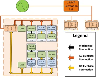
system. Due to the nonlinearities in the FREEDM system, the modeling process starts with building sub-system state-space models, such as those for SST, Wind DRER, PV DRER and DESD. The sub-system models are then integrated to build the comprehensive FREEDM system model. The component states and the associated controller states are also separated such that the plant model and the controller model can be developed and upgraded individually. The functional diagram representing the FREEDM system that includes SST and other sub-systems considered for the modeling purpose are shown in Fig. 2.1. In Fig. 2.2, all the parameters and physical states are shown by 𝑎_𝑖 and 𝑥_𝑖, respectively; PI controller states are denoted by ξ_𝑖; and 𝑑_𝑖’s are the output of the controllers. DAB output current is denoted by 𝐼_𝐷𝐴𝐵, rectifier net output power is presented by 𝑃_𝑟𝑒𝑐, while 𝐿_𝐷𝐶 and 𝐿_𝐴𝐶 represent the net load of DC and AC energy cells (generation sources, energy storage and local loads), respectively. The time-scales of evolution of the different states, however, are sharply different ranging from 10-3 microseconds to 0.1 seconds within SST. Singular perturbation techniques have been applied to reduce the model order, and represent it in a more tractable form. Singular perturbation method separates the dynamic system into slow and fast variables that allow the simplification of the rectifier model by eliminating the states those have no effects on system performance [46]. Total system states have been reduced from more than hundreds for the full FREEDM system by utilizing the singular perturbation technique and that makes the system analysis simpler. The final order of the simplified derived model, including all internal controller states, is seventy.

2.2.1 SST - Rectifier Model and Controllers

(32)

represent an L-rectifier through model reduction. In a dual loop controller, the rectifier output voltage is controlled in the outer loop that generates the d-axis current reference for controlling the 𝑖_𝑑-component of the SST input current in the inner loop. Current reference can be set to zero for unity power factor in the q-axis controller that controls the reactive power flow.

Fig. 2.2 shows the simplified circuit diagram of the rectifier and the equations (2.1)-(2.10) present the rectifier physical states, controller states and controller output where 𝑦₁, 𝑦₂,

𝑥1and 𝑥2 represent d and q-axes grid voltages and currents, respectively. All the parameters

and states are enlisted in table 1.1.

𝑥̇₁ = −𝑎2

𝑎1𝑥1+ 𝜔1𝑥2+

1

𝑎1𝑑1𝑥3 −

1

𝑎1𝑦1 (2.1) 𝑥̇₂ = −𝜔₁𝑥₁−𝑎2

𝑎₁𝑥2+ 1

𝑎₁𝑑2𝑥3− 1

𝑎₁𝑦2 (2.2)

𝑥̇3 = −

1 2𝑎3

𝑑𝑎𝑥𝑎 −

𝑃_𝑟𝑒𝑐 𝑎3𝑥3

(2.3)

𝑑𝑎 and 𝑥𝑎 can be found using equations (2.4-2.5) through inverse dq-αβ modeling and the

(33)

Load DRER Generator Wind Turbine DRER PV

DC to DC Converter

DESD DC to DC Converter Battery DRER Generator Wind Turbine Load DESD

DC to AC Inverter

Battery

DRER

PV DC to AC

Inverter SST with Energy Cell SST with Energy Cell

1 MVA Substation SST

Legend

Mechanical Connection AC Electrical Connection DC Electrical Connection

AC to DC Rectifier Re cti fi er D A B In ver ter SST Rec ti fi er D A B In ver ter SST Rec ti fi er D A B In ver ter SST

Figure 2.1. One node FREEDM system model.

𝑑_𝑎 = 𝑑₁cos(𝜃) + 𝑑₂sin(𝜃) (2.4)

𝑥𝑎 = 𝑥1cos(𝜃) + 𝑥2sin(𝜃) (2.5)

ξ̇1 = 𝑟1− 𝑥3 (2.6)

ξ̇₂ = 𝑎₄(𝑟₁− 𝑥₃) + 𝑎₅ξ₁− 𝑥₁ (2.7)

ξ̇3 = 𝑞1− 𝑥2 (2.8)

𝑑₁ = 𝑎₆(𝑎₄(𝑟₁− 𝑥₃) + 𝑎₅ξ₁− 𝑥₁) + 𝑎₇ξ₂ (2.9)

𝑑₂ = 𝑎₈(𝑞₁− 𝑥₂) + 𝑎₉ξ₃ (2.10)

2.2.2 SST - DAB Model and Controllers

(34)

are input and output capacitor voltages and inductor current. However, the system can be divided into a slow-varying system and a fast-varying system since the capacitor voltage changes are much slower compared to the changes in inductor current [47, 48].

a10 a12 a15 a11 H1 1:a13 H2

x4 a18a19

a20

x8,x9

x6,x7

+

-y1,y2 a2 _a₃ _x

3

x1,x2

a1 ₊

- x5 LDC LAC

+ -+ -DAB RECTIFIER _INVERTER IDAB

Figure 2.2. Solid-state transformer circuit model.

The two-dimensional representation of the DAB converter is obtained by linearly representing the fast-varying inductor current in each sub-interval and applying the state-space averaging method. Equations (2.11) - (2.14) provide the final state models for DAB along with the controller output.

𝑥̇4 = + 1

𝑎10𝑎12𝑥3−

1

𝑎10𝑎12𝑥4−

𝜙3(1−𝜙3)𝑎13

2𝑎10𝑎14𝑎15 𝑥5 (2.11) 𝑥̇₅ = 𝜙3(1−𝜙3)𝑎13

2𝑎11𝑎14𝑎15 𝑥4−

1

𝑎11𝐿𝐷𝐶𝑥5 (2.12)

ξ̇₄ = 𝑟₂− 𝑥₅ (2.13)

𝜙₃ = 𝑎₁₆(𝑟₂− 𝑥₅) + 𝑎₁₇ξ₄ (2.14)

2.2.3 SST - Inverter Model and Controllers

(35)

where 𝑥₆, 𝑥₇, 𝑥₈ and 𝑥₉ represent d and q -axes inverter output currents and voltages, respectively.

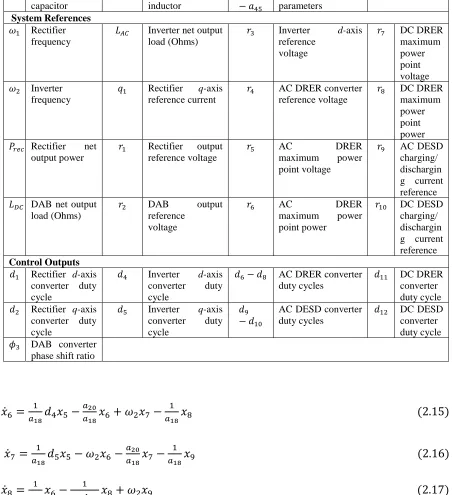
Table 2.1. FREEDM system parameter list.

System and Controller States 𝑥1 Rectifier d-axis

inductor current

𝑥7 Inverter q-axis

inductor current

𝑥25 − 𝑥30

DC DESD interface converter states

ξ13 DC DRER

interface converter controller state

𝑥2 Rectifier q-axis

inductor current

𝑥8 Inverter d-axis

capacitor voltage

ξ1−ξ3 Rectifier controller

states

ξ14 DC DESD

interface converter controller states

𝑥3 Rectifier capacitor

voltage

𝑥9 Inverter q-axis

capacitor voltage

ξ4 DAB controller

state

𝑥4 DAB input

capacitor voltage

𝑥10 − 𝑥15

AC DRER interface

converter states

ξ5−ξ6 Inverter controller

states

𝑥5 DAB output

capacitor voltage

𝑥16 − 𝑥21

AC DESD interface

converter system states

ξ7−ξ10 AC DRER interface

converter controller states

𝑥6 Inverter d-axis

inductor current

𝑥22 − 𝑥24

DC DRER interface

converter states

ξ7−ξ10 AC DESD interface

converter controller states

System Parameters 𝑎1 Rectifier filter

inductor

𝑎11 DAB output

capacitor

𝑎19 Inverter filter

capacitor

𝑎46 − 𝑎47

DC DRER interface converter controller gains

𝑎2 Rectifier filter

resistor

𝑎12 DAB input

resistor

𝑎20 Inverter input filter

resistor

𝑎48 − 𝑎57

AC DESD physical parameter s

𝑎3 Rectifier capacitor 𝑎13 Transformer turns

ratio

𝑎21, 𝑎22 Inverter d-axis

gains of controller

𝑎58 − 𝑎61

AC DESD interface converter controller gains

𝑎4, 𝑎5

Rectifier gains of voltage controller

𝑎14 Transformer

switching frequency

𝑎23, 𝑎24 Inverter q-axis

gains of controller

𝑎62 − 𝑎75

DC DESD physical parameter s

𝑎6, 𝑎7

Rectifier d-axis gains of controller

𝑎15 Transformer

inductor

𝑎25 − 𝑎33

AC DRER physical parameters

𝑎76 − 𝑎77

DC DESD converter controller gains

𝑎8, 𝑎9

Rectifier q-axis gains of controller

𝑎16, 𝑎17

DAB PI controller gains

𝑎34 − 𝑎41

(36)

Table 2.1 Continued

𝑎10 DAB input

capacitor

𝑎18 Inverter filter

inductor

𝑎42 − 𝑎45

DC DRER physical parameters

System References 𝜔1 Rectifier

frequency

𝐿𝐴𝐶 Inverter net output

load (Ohms)

𝑟3 Inverter d-axis

reference voltage

𝑟7 DC DRER

maximum power point voltage

𝜔2 Inverter

frequency

𝑞1 Rectifier q-axis

reference current

𝑟4 AC DRER converter

reference voltage

𝑟8 DC DRER

maximum power point power

𝑃𝑟𝑒𝑐 Rectifier net

output power

𝑟1 Rectifier output

reference voltage

𝑟5 AC DRER

maximum power point voltage

𝑟9 AC DESD

charging/ dischargin g current reference

𝐿𝐷𝐶 DAB net output

load (Ohms)

𝑟2 DAB output

reference voltage

𝑟6 AC DRER

maximum power point power

𝑟10 DC DESD

charging/ dischargin g current reference

Control Outputs 𝑑1 Rectifier d-axis

converter duty cycle

𝑑4 Inverter d-axis

𝑑6− 𝑑8 AC DRER converter

duty cycles

𝑑11 DC DRER

𝑑2 Rectifier q-axis

𝑑5 Inverter q-axis

𝑑9 − 𝑑10

AC DESD converter duty cycles

𝑑12 DC DESD

𝜙3 DAB converter

phase shift ratio

𝑥̇₆ = 1

𝑎18𝑑4𝑥5−

𝑎20

𝑎18𝑥6+ 𝜔2𝑥7−

1

𝑎18𝑥8 (2.15) 𝑥̇₇ = 1

𝑎18𝑑5𝑥5 − 𝜔2𝑥6−

𝑎20

𝑎18𝑥7−

1

𝑎18𝑥9 (2.16)

𝑥̇₈ = 1

𝑎19𝑥6−

1

𝑎19𝐿𝐴𝐶𝑥8+ 𝜔2𝑥9 (2.17) 𝑥̇₉ = 1

𝑎19𝑥7− 𝜔2𝑥8−

1

𝑎19𝐿𝐴𝐶𝑥9 (2.18)

ξ̇₅ = 𝑦₃ − 𝑥₈ (2.19)

(37)

𝑑₄ = 𝑎₂₁(𝑦₃− 𝑥₈) + 𝑎₂₂ξ₅ (2.21)

𝑑₅ = 𝑎₂₃(𝑦4− 𝑥9) + 𝑎24ξ6 (2.22)

2.2.4 DRER Model and Controllers

(38)

to amplify the panel voltage to DC bus voltage. Based on voltage level of the panels, other DC-DC converters can also be coupled for the interface. Mathematical model for the interface is also developed and shown in equations (2.36)-(2.40).

𝑥̇₁₀ = 1

𝑎25𝑥11−

1−𝑑6

𝑎25 𝑥12 (2.23) 𝑥̇₁₁ = − 1

𝑎26𝑥10+

1 𝑎26

𝑢2

𝑥11 (2.24) 𝑥̇₁₂ =1−𝑑6

𝑎27 𝑥10−

1

𝑎27𝑎28𝑥12+

1

𝑎27𝑎28𝑥15 (2.25) 𝑥̇13 = −

1 𝑎31𝑥8−

𝑎33

𝑎31𝑥13+ 𝜔2𝑥14+

1

𝑎31𝑑7𝑥15 (2.26) 𝑥̇14 = −

1

𝑎31𝑥9− 𝜔2𝑥13−

𝑎33

𝑎31𝑥14+

1

𝑎31𝑑8𝑥15 (2.27) 𝑥̇₁₅ = − 1

2𝑎₃₂𝑑7𝑥13− 1

2𝑎₃₂𝑑8𝑥14− 1 𝑎₃₂

𝑢₂

𝑥₁₅ (2.28)

ξ̇7 = 𝑢1− 𝑥11 (2.29)

x

22

a

44

x

₂₄

+

-a

45

x

5

+

-a

42

a

43

+

_-

_x

₂₃

S

1

D

1

I

MPP

Figure 2.4: PV DRER and boost converter for PV DC interface.

x10

a27 x12

+

-a28

a25

a26 +_-_x11 S1

D1

x13,x14

a31 a33 +

-_x15a32 x8,x9

IMPP

BOOST _Rectifier

(39)

ξ̇₈ = 𝑟₃− 𝑥₁₅ (2.30)

ξ̇9 = 𝑎34(𝑟3− 𝑥15) + 𝑎35ξ8− 𝑥13 (2.31)

ξ̇₁₀= −𝑥₁₆ (2.32)

𝑑₆ = 𝑎₃₆(𝑢₁− 𝑥₁₁) + 𝑎₃₇ξ₇ (2.33)

𝑑₇ = 𝑎₃₈(𝑎34(𝑟3− 𝑥15) + 𝑎35ξ8 − 𝑥13) + 𝑎39ξ9 (2.34)

𝑑₈ = −𝑎₄₀𝑥₁₆+ 𝑎₄₁ξ₁₀ (2.35)

𝑥̇₂₂ = 1

𝑎42𝑥23−

(1−𝑑11)

𝑎42 𝑥24 (2.36) 𝑥̇₂₃ = − 1

𝑎43𝑥22+

𝑢4

𝑎43𝑥23 (2.37) 𝑥̇₂₄ =(1−𝑑11)

𝑎44 𝑥22−

1

𝑎44𝑎45𝑥24+

1

𝑎44𝑎45𝑥5 (2.38)

ξ̇₁₃= 𝑢₃− 𝑥₂₃ (2.39)

𝑑₁₁ = 𝑎₄₆(𝑢3− 𝑥23) + 𝑎47ξ13 (2.40)

2.2.5 DESD Model and Controllers

(40)

DESD model for the FREEDM system has utilized the detailed storage modeling to capture all the transients [51, 52]. Similar to the DRER, the DESD controller objective is to match the output voltage with AC bus voltage.

𝑥̇₁₆ = − 1

𝑎48𝑥8−

𝑎50

𝑎48𝑥16+ 𝜔2𝑥17+

1

𝑎50𝑑9𝑥18 (2.41) 𝑥̇₁₇ = − 1

𝑎48𝑥9− 𝜔2𝑥16−

𝑎50

𝑎48𝑥17+

1

𝑎48𝑑10𝑥18 (2.42)

𝑥̇18 =−

1

2𝑎₄₉𝑑9𝑥16− 1

2𝑎₄₉𝑑10𝑥17− 1

𝑎₄₉𝑎₅₁𝑥18+ 1

𝑎₄₉𝑎₅₁∗ (𝑉𝑜𝑐+ 𝑥20+ 𝑥21− 𝑥18) (2.43)

𝑥̇₁₉ = − 1

𝑎₅₂𝑎₅₃𝑥19+

1

𝑎₅₂(𝑎₅₁+ 𝑎₅₀)∗ (𝑉𝑜𝑐+ 𝑥20+ 𝑥21− 𝑥18) (2.44)

𝑥̇₂₀ = − 1

𝑎54𝑎55𝑥20+

1

𝑎54(𝑎51+𝑎50)∗ (𝑉𝑜𝑐+ 𝑥20+ 𝑥21− 𝑥18) (2.45)

𝑥̇₂₁ = − 1 𝑎56𝑎57

𝑥₂₁+ 1

𝑎56(𝑎51+ 𝑎50)

∗ (𝑉_𝑜𝑐+ 𝑥₂₀+ 𝑥₂₁− 𝑥₁₈) (2.46)

ξ̇₁₁= 𝑢₅− 𝑥₁₆ (2.47)

ξ̇₁₂= −𝑥₁₇ (2.48)

𝑑9 = 𝑎58(𝑢5− 𝑥16) + 𝑎59ξ11 (2.49)

𝑑₁₀ = −𝑎₆₀𝑎₁₇+ 𝑎₆₁ξ₁₂ (2.50)

(41)

+

- - + - +

a53 a52

Ibat

x19

+

- Voc

a50 a55

a54

x20 x21

a56 a57 a49 +_x 18 -DESD

x16,x17

a48 a50

x8,x9

Rectifier a51

Figure 2.5: DESD and rectifier circuit for AC DESD average model.

+

- - + - +

a69 a68

Ibat

x28

+

- Voc

a67 a73

a72

x29 x30

a74

a75 a66

a65

+_x

27

S1 D1

a62 a63 _x 26 + -a64 x5 + -x25 DESD BUCK-BOOST

Figure 2.6: DESD and buck-boost circuit for DC DESD average model.

𝑥̇26 = 1

𝑎63𝑎64𝑥5−

(1−𝑑12)

𝑎63 𝑥25−

1

𝑎63𝑎64𝑥26 (2.51) 𝑥̇₂₇ = −𝑑12

𝑎₆₅𝑥25+

(1 − 𝑑12)

𝑎₆₅(𝑎66+ 𝑎67)

∗ (𝑉_𝑜𝑐+ 𝑥₂₉+ 𝑥₃₀− 𝑥₂₇) (2.52)

𝑥̇28 = −

1 𝑎68𝑎69

𝑥28−

1

𝑎68(𝑎66+ 𝑎67)

∗ (𝑉𝑜𝑐+ 𝑥29+ 𝑥30− 𝑥27) (2.53)

𝑥̇29 = − 1

𝑎72𝑎73𝑥29+

1

𝑎72(𝑎68+𝑎69)∗ (𝑉𝑜𝑐+ 𝑥29 + 𝑥30− 𝑥27) (2.54) 𝑥̇₃₀ = − 1

𝑎₇₄𝑎₇₅𝑥30+

1

𝑎₇₄(𝑎66+ 𝑎67)

∗ (𝑉_𝑜𝑐+ 𝑥₂₉ + 𝑥₃₀− 𝑥₂₇) (2.55)

ξ̇14= 𝑢6−

(𝑥₅− 𝑥₂₆)

𝑎₆₄ (2.56)

𝑑₁₂ = 𝑎₇₅(𝑢₆−(𝑥5− 𝑥26)

(42)

2.3. Case Studies with the Developed Average Model

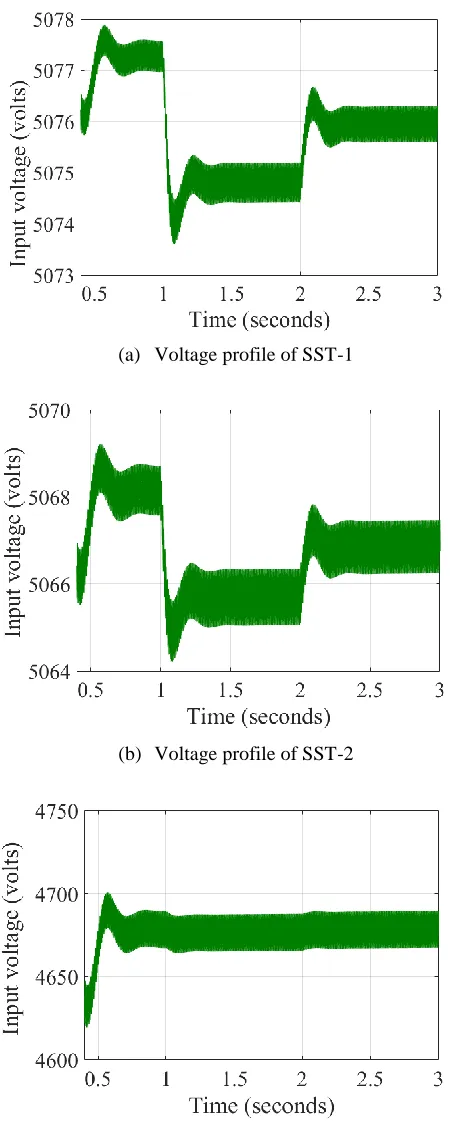
Several case studies have been conducted with the developed comprehensive FREEDM system model to evaluate the impact on the output voltage levels in different stages of the system and track performance for the controller setpoints. Results are observed where DC and AC buses are maintained at the set voltage levels with load changes in DC or AC energy cells, start/stop of DRER generation and DESD charging/discharging modes. Summary results of two particular cases are shown in Fig. 2.7. Fig. 2.7 (a) shows that PV generation of 0.5 kW added at t=1 sec from the DC energy cells causes an overshoot in the SST rectifier, DAB and inverter output voltages with energy being fed back to the grid. The energy storage in the charging mode and wind generation unit are connected to the system at t=2 secs and 3.2 secs, respectively. The DC voltage in rectifier and DAB output drops at first, but the controllers are able to maintain the steady-state regulation, also inverter output voltage experiences voltage sag for a shorter time due to faster timescale of the controller. For analyzing the dynamics introduced by the AC energy cell, PV DRER, AC DESD, and wind generation are connected to the system at t=5 secs, 6 secs and 7.2 secs, respectively. Fig. 2.7 (b) shows that the DC bus voltage along with inverter output fluctuates due to addition of the AC energy cell components. Fig. 2.8 shows the system response when the SST operating mode is changed for reversing the power flow with renewable generation and active load reduction. DC bus voltage of the rectifier and DAB show overshoot before settling to the desired regulation points within 0.3 secs.

(43)

(44)

(a)

(b)

(45)

Figure 2.8: Case study with regenerative mode of operation.

(46)

Figure 2.10: Case study with active power variation.

(47)

2.4. Feasibility and Stability Surface Plots Based on Rectifier Model

The 70th-order nonlinear differential-algebraic state-space model of a single-SST FREEDM power distribution system developed in the previous sections provides the opportunity to derive analytical relationships between physical parameters and feasible operational range. Nonlinear differential-algebraic state-space model of SST developed in the previous sections provides the opportunity to analyze the relationship as previous studies have shown a possible failure in the SST-based power distribution system in the SST farthest from the grid [28]. However, there is no indication of the reason for the failure; since the grid in the simulations has been assumed to be an infinite grid, the system breakdown can be either due to infeasibility or instability. Addressing this issue is one of the research motivation as that will eventually figure out the power bounds of such system, if there is any. Once the feasibility bounds are found for SST, the system parameters can be designed accordingly to provide the required power flow and energy exchange flexibility. Feasibility analysis of the FREEDM system is essential to answer the maximum net power capability that the system can handle. Once the feasibility bounds are known, the system parameters can be designed accordingly to provide the required power flow and energy exchange flexibility. The pair (𝑦₁, 𝐼_𝐷𝐴𝐵) has been identified to be critical for determining the equilibrium of the nonlinear FREEDM model where 𝐼𝐷𝐴𝐵 represents the net current flowing through the DAB and 𝑦1 is

(48)

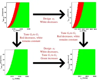
operation region for any pair of (𝑦₁, 𝐼_𝐷𝐴𝐵). Fig. 2.12 shows that reducing 𝑎₂ results in expansion of feasible operating region of SST (green, red and white colors indicate the feasible stable, feasible unstable and infeasible region, respectively). It has also been found through analysis that proper choice of the rectifier output DC voltage reference can extend the feasibility bounds of the SST.

𝑥1,𝑠𝑠 =

−_𝑎𝑦1

2± √(

𝑦₁ 𝑎2)

2₋8𝐼𝐷𝐴𝐵,𝑠𝑠𝑟2

𝑎2

2 (2.58)

𝐼_{𝐷𝐴𝐵,𝑠𝑠}≤ 𝑦1

2

8𝑎₂𝑟₂ (2.59)

Figure 2.12. Expansion of feasibility region by reducing rectifier resistance.

Red zones represent the unstable regions inside the feasible operational range which can be reduced with the proper tuning of the controller gains. Fig. 2.13 shows the circular relationship between the system parameters and controller gains with the feasibility and stability region, respectively.

(49)

Design a2

White decreases

Tune G0 to G1

Red decreases, white remains constant

Tune G0 to G2

Red decreases, white remains constant

Design a2

White decreases, Tune G1 to G2

Green increases

Figure 2.13. Feasibility and stability circle diagram.

Figure 2.14. Expansion of stability region by retuning the controller gains.

Fig. 2.14 presents a case of the controller tuning to show the expansion of the feasible and stable region.

(50)

2.5. Contribution

1. Comprehensive average model of the FREEDM system that includes the SST and energy cells. PV, wind and storage make up the energy cells in the DC and AC buses.

2. Operational bounds for the SST based system to guarantee the feasible operation. The bounds are studied with a simplified SST model with rectifier states and surface plots clearly show the feasible and infeasible regions. Later, controller gains are also tuned to see the impact on the stability of the feasible operational points.

2.6. Conclusions

(51)

CHAPTER 3 POWER SHARING METHODS IN A MULTIPLE SST BASED

SYSTEM

3.1. Introduction

3.2. Single SST Feasibility Constraints and Expansion to Multi-SST Case 3.3. Proposed Power Sharing Methods to Maintain Feasibility

3.4. Case Studies with Different Conditions to Verify the Proposed Methods 3.5. Formulation of IPM/IEM Control Separation Based on the Study 3.6. Contribution

(52)

3.1 . Introduction

(53)

(54)

3.2. Single SST Feasibility Constraints and Expansion to Multi-SST

Case

In this section, a feasibility analysis problem is formulated to find permissible total load that each part of the SST can handle (assuming infinite generation). Dynamic model and duty cycle constraint neglecting the second order grid harmonics for each SST subsystem can be written as equation (3.1) and (3.2), where 𝛼1and 𝛼3are the system parameters and references,

respectively and 𝛼₂ ≜ {𝐿∗_𝑑𝑐= 𝐿_𝑑𝑐(𝑡 → ∞), 𝐿∗_𝑎𝑐 _{= 𝐿}

𝑎𝑐(𝑡 → ∞) } represents the steady-state

value of net loads of DC and AC energy cells, respectively.

𝑓(𝑥̅, 𝛼1, 𝛼2, 𝛼3) = 0 (3.1)

𝑔(𝑥̅, 𝛼₁, 𝛼₂, 𝛼₃) ≤ 0 (3.2)

Dynamical model of a SST coupled to the models of the DC and AC energy cells in the low voltage distribution side is derived in previous chapter. The energy cells comprise of local loads, renewable generation (photovoltaic and/or wind power), and storage devices. Functional FREEDM system with SSTs connected in a tree topology is shown in Fig. 3.1; the circuit diagram of the SST model is provided in Fig. 3.2.

3.2.1. Feasibility Analysis of Rectifier

(55)

(3.4).

𝑦1 = 𝑣𝑔𝑟𝑖𝑑+ 𝑅𝑙𝑖𝑛𝑒1𝑥1 − 𝑋𝑙𝑖𝑛𝑒1𝑥2 (3.3)

𝑦₂ = 𝑅_{𝑙𝑖𝑛𝑒1}𝑥₂+ 𝑋_{𝑙𝑖𝑛𝑒1}𝑥₁ (3.4)

SST-3

DC Load Generation Storage AC Load Generation Storage

SST-2

DC Load Generation Storage AC Load Generation Storage

SST-1

DC Load Generation Storage AC Load Generation Storage PCC Rest of the Grid

z

line,1

z

line,2

z

line,3

Figure 3.1: FREEDM system functional diagram.

a10

a12

a15 a₁₁

1:a13

x4

a18

a19

a20

x8, x9

x6, x7

+

-y1, y2

a2

a3 x3

x1, x2

a1 ₊

- x5 Ldc Lac

+ -+ -DAB RECTIFIER INVERTER IDAB + -+

-Figure 3.2: Circuit diagram of a solid-state transformer.

System states of the rectifier can be formulated as an equation of circle as shown in (3.5).

(𝑥₁+ 𝑦1 2𝑎₂)

2

+ (𝑥₂ + 𝑦2 2𝑎₂)

2

= 𝑦1

2_{+ 𝑦}

22

4𝑎₂2 − 2𝑃_𝑟𝑒𝑐

𝑎₂ (3.5)

Based on the radius of the equation (3.5), the maximum power that can be processed through the rectifier stage of the SST is derived in (3.6).

𝑃_{𝑟𝑒𝑐,𝑚𝑎𝑥}= 𝑦1

2_{+ 𝑦}

22

(56)

As the rectifier has power electronics switches and it requires to follow the duty cycle constrains and that can be formulated as an inequality equation as in (3.7).

(𝑥1 +

𝑎₂𝑦₁+ 𝑎₁𝜔₁𝑦₂ 𝑎₂2_{+ 𝑎}

12𝜔12

)

2

+ (𝑥2+

𝑎₂𝑦₂− 𝑎₁𝜔₁𝑦₁ 𝑎₂2_{+ 𝑎}

12𝜔12

)

2

≤ 𝑟1

2

𝑎₂2_{+ 𝑎} 12𝜔12

. (3.7)

Therefore, the feasibility range of the rectifier is defined as all of the points on the circle given in equation (3.5) that are on or inside the inequality equation given in (3.7). The constraints developed in equation (3.5) is dependent on the net power requirement of each SST and it can be extended to multi-SST case to analyze the feasibility in a microgrid. Feasibility analysis is first extended for multi-SST case considering the rectifier model only and then, the power sharing methods are developed based on that.

3.2.2. Multi-SST Circle Condition to Maintain Feasibility

(57)

Figure 3.3. Simplified tree configuration with multi-SST.

The 3-SST configuration is used as benchmark for the analytical analysis and further simulation validation. Generally, in an n-SST distribution system, aside from the convergence of the power flow solution, there are n constraints that need to be satisfied. It should be noted that the solution of the power flow, i.e., the input voltages of each SST in the system is dependent on the net power of all of the SSTs in a network and that will impact the feasibility range. This is the coupling effect of SST loads on the input voltage of any neighboring SSTs. The feasibility constraints in this case will be similar as in equations (3.5) and (3.7) with the exception that the input voltages are not anymore free variable. Input voltage of any SST is expressed in equation (3.10). Feasibility equations for multi-SST cases are given in equations (3.8) and (3.9). The physical meanings of the states are the same as in section 3.2; the subscript 𝑖 denotes the 𝑖𝑡ℎ_{SST, where}_{𝑖 = 1,2,3, … . . , 𝑛}_and_𝑍

𝑙𝑖𝑛𝑒,𝑖 refers to

𝑖𝑡ℎSST the line impedance.

(𝑥1𝑖+

𝑦_1𝑖 2𝑎2𝑖

)

2

+ (𝑥2𝑖+

𝑦_2𝑖 2𝑎2𝑖

)

2

=𝑦1𝑖

2_{+ 𝑦}

2𝑖2

4𝑎2𝑖2

−2𝑃𝑟𝑒𝑐,𝑖 𝑎2𝑖

(3.8)

(𝑥_1𝑖+𝑎2𝑖𝑦1𝑖+ 𝑎1𝑖𝜔1𝑖𝑦2𝑖 𝑎_2𝑖2 + 𝑎_1𝑖2𝜔_1𝑖2 )

2

+ (𝑥_2𝑖+𝑎2𝑖𝑦2𝑖− 𝑎1𝑖𝜔1𝑖𝑦1𝑖 𝑎_2𝑖2 + 𝑎_1𝑖2𝜔_1𝑖2 )

2

≤ 𝑟1𝑖

2

(58)

𝑦_1𝑖+ 𝑗 ∗ 𝑦_2𝑖 = 𝑣_{𝑔𝑟𝑖𝑑}

+ 𝑍_{𝑙𝑖𝑛𝑒1}∑ (𝑥_1𝑘+ 𝑗𝑥_2𝑘) + 𝑍𝑙𝑖𝑛𝑒2∑ (𝑥1𝑘 + 𝑗𝑥2𝑘)

𝑛

𝑘= 2

+ ⋯

𝑛

𝑘= 1

+ 𝑍_{𝑙𝑖𝑛𝑒𝑖}∑(𝑥_1𝑘+ 𝑗𝑥_2𝑘)

𝑛

𝑘= 𝑖

(3.10)

3.3. Proposed Power Sharing Methods to Maintain Feasibility

In this section, power sharing methods are analyzed for properly updating the input current setpoints of each SST whenever there is a change in the load demand of one of the SSTs. Our goal is to find the maximum allowable change in the power that can flow through any

𝑖𝑡ℎSST, due to such a change in the load so that the overall system can remain within a feasible zone of operation. A follow-up question is how should the input references of each SST change to handle this change in power flow? The envisioned architecture of the FREEDM distribution grid model consists of two layers of decision-making units - namely, IEM and IPM. The IEM layer is responsible for generating accurate load forecasts based on weather data, economic dispatch, and feedback information from various customers through their smart meter data, etc., over an interval of every 15 to 20 minutes. The IPM, on the other hand, is responsible for regulating the DC and AC link output voltages and input currents of each SST to comply with any change in the load. Loads can change through three distinct scenarios, as follows and is shown in Fig. 3.4:

Case 0: Unpredicted small changes in load

(59)

these bounds then the internal control methods such as droop control or small manipulations in the power generated by the batteries connected to this SST can maintain feasible operation of the system without any further need for updating the current setpoints.

IEM Command 1

time power

Case 0

Case 1 Case 2

IEM Command 2 IEM Command 3

Figure 3.4. Different cases with change in power.

Case 1: Unpredicted large changes in load

If the load changes suddenly by a large amount in an unpredicted fashion then neither droop control will be able to compensate for this large change neither IPM will have enough time to recalculate the setpoints by solving a large power flow problem. In this situation, the IPM must override the IEM commands instantaneously to maintain the feasibility of the system. We next state two power sharing methods between SSTs by which this can be made possible.

Case 2: Predicted large changes in load

(60)

power flow algorithm for the entire grid model over this 15 minute interval, and compute new setpoints for the voltages and currents of every SST.

3.3.1. Method 1: Power Sharing with Constant Input Current

In order to avoid the complexity of running power flow algorithms as in Case 1 when there is a change in power of a SST, other SSTs can help the SST in need by reducing their net power while keeping their input current setpoint the same as before. Net power of the neighboring SSTs has to satisfy the maximum power constraints with their updated input voltages. Firstly the circle expression for the multiple SSTs according to equation 3.8 to 3.10 are considered to maintain the feasibility in developing these power sharing methods. The node voltage of the SSTs are expressed in equation (3.11) for a radial network of FREEDM system as shown in Fig. 3. 5.

z

1g SST1

z

(i-1)i SSTi-1

z

i(i+1) SSTi

z

n SSTn

MVAC vg

Vi (αi* ) Vn (αn* )

Vi-1 (αi-1* )

V1 (α1* )

Ii

Ii-1

I1 In

Figure 3.5. Radial network of FREEDM system.

𝑉₁ = 𝑉_𝑔− 𝑍₁(𝐼₁+ 𝐼₂+. . +𝐼_𝑖+. . +𝐼_𝑛)

𝑉₂ = 𝑉₁− 𝑍₂(𝐼₂+. . +𝐼_𝑖+. . +𝐼_𝑛)

……….. ………..

𝑉_𝑖−1 = 𝑉_𝑖−2− 𝑍_𝑖−1(𝐼_𝑖−1+ 𝐼_𝑖+. . +𝐼_𝑛)

𝑉𝑖 = 𝑉𝑖−1− 𝑍𝑖(𝐼𝑖 + 𝐼𝑖+1+. . +𝐼𝑛)

(61)

𝑉_𝑛 = 𝑉_𝑛−1− 𝑍_𝑛𝐼_𝑛 (3.11)

With a change in power in the 𝑖𝑡ℎ SST, the current of that SST will change and other will also change due to the subsequent change in the voltage if the net power remains the same in all the other SSTs in the network as shown in equation (3.12).

𝑉₁′= 𝑉_𝑔′− 𝑍₁(𝐼₁′ + 𝐼₂′+. . +𝐼_𝑖′+. . +𝐼_𝑛′)

𝑉₂′ = 𝑉₁′− 𝑍2(𝐼2′+. . +𝐼𝑖′+. . +𝐼𝑛′)

……….. ………..

𝑉_𝑖−1′ = 𝑉_𝑖−2′ − 𝑍𝑖−1(𝐼𝑖−1′ + 𝐼𝑖′+. . +𝐼𝑛′)

𝑉_𝑖′= 𝑉_𝑖−1′ − 𝑍_𝑖(𝐼_𝑖′+ 𝐼_𝑖+1′ +. . +𝐼_𝑛′₎

……….. ………..

𝑉_𝑛−1′ = 𝑉_𝑛−2′ − 𝑍𝑛(𝐼𝑛−1′ + 𝐼𝑛′)

𝑉_𝑛′= 𝑉_𝑛−1′ − 𝑍_𝑛𝐼_𝑛′ (3.12)

However, the system will never reach to solution without a power flow solver if all the node voltage and currents are getting changed and the system will become oscillatory. Power flow solver has a significant computation delay which is impractical to run during the IPM operation. To avoid the complexity of running the power during the IEM commands, in method one the node current of the other SSTs except the 𝑖𝑡ℎ_{SST remain unchanged as}

shown in equation (3.13).

𝑉₁′= 𝑉_𝑔′_{− 𝑍}

1(𝐼1 + 𝐼2+. . +𝐼𝑖′+. . +𝐼𝑛)

𝑉₂′ = 𝑉₁′− 𝑍2(𝐼2+. . +𝐼𝑖′+. . +𝐼𝑛)

(62)

………..

𝑉_𝑖−1′ = 𝑉_𝑖−2′ − 𝑍𝑖−1(𝐼𝑖−1+ 𝐼𝑖′+. . +𝐼𝑛)

𝑉_𝑖′= 𝑉_𝑖−1′ − 𝑍_𝑖(𝐼_𝑖′+ 𝐼_𝑖+1+. . +𝐼_𝑛)

𝑉_𝑖+1′ = 𝑉_𝑖′− 𝑍𝑖+1(𝐼𝑖+1+ 𝐼𝑖+2+. . +𝐼𝑛)

……….. ………..

𝑉_𝑛−1′ = 𝑉_𝑛−2′ − 𝑍_𝑛(𝐼_𝑛−1+ 𝐼_𝑛)

𝑉_𝑛′_{= 𝑉}

𝑛−1′ − 𝑍𝑛𝐼𝑛 (3.13)

It can be shown from equations (3.11) to (3.13), to maintain the current of each nodes same as before; the voltage difference of each node will be a function of the change in current of

𝑖𝑡ℎ SST and is shown in equations (3.14) – (3.15).

𝛥𝑉_𝑚= 𝛥𝑉_𝑖; 𝑓𝑜𝑟 𝑚 ∈ {1, … … . . , 𝑛} ≠ 𝑖 (3.14)

𝛥𝑦_1𝑚+ 𝑗𝛥𝑦_2𝑚 = 𝛥𝑦_1𝑖+ 𝑗𝛥𝑦_2𝑖 = (∆𝑥_1𝑖+ 𝑗∆𝑥_2𝑖) ∑ 𝑟_𝑘+ 𝑗 𝑥_𝑘

𝑚

𝑝=1

(3.15)

Assuming that the q-axis input current of 𝑆𝑆𝑇𝑖 remains unchanged (𝑥2𝑖′ = 𝑥2𝑖), the change in

𝑥_1𝑖 can be found by reducing the feasibility equations given by (3.8) for the two conditions before and after the change. This would result in a second order polynomial shown in (3.16) relating the change in d-axis current of 𝑆𝑆𝑇𝑖 (∆𝑥1𝑖) to the change in the net power (∆𝑃𝑟𝑒𝑐,𝑖),

system parameters, and current operating point of the system.

(𝑎_2𝑖+ ∑ 𝑅_{𝑙𝑖𝑛𝑒,𝑘}

𝑖

𝑘=1

) ∆𝑥_1𝑖2+ {2𝑎_2𝑖𝑥_1𝑖+ 𝑦_1𝑖+ ∑ 𝑅_{𝑙𝑖𝑛𝑒,𝑘}

𝑖

𝑘=1

𝑥_1𝑖+ ∑ 𝑋_{𝑙𝑖𝑛𝑒,𝑘}

𝑖

𝑘=1

𝑥_2𝑖} ∆𝑥_1𝑖

(63)

The maximum allowable change in the power (∆𝑃_{𝑟𝑒𝑐,𝑖}_𝑚𝑎𝑥) can be found based on the discriminant of this equation.

∆𝑃_{𝑟𝑒𝑐,𝑖}_𝑚𝑎𝑥 = {2𝑎2𝑖𝑥1𝑖+ 𝑦1𝑖+ ∑ 𝑅𝑙𝑖𝑛𝑒,𝑘

𝑖

𝑘=1 𝑥1𝑖+ ∑𝑖𝑘=1𝑋𝑙𝑖𝑛𝑒,𝑘𝑥2𝑖}

2

8(𝑎_2𝑖+ ∑𝑖_𝑘=1𝑅_{𝑙𝑖𝑛𝑒,𝑘}) (3.17)

Since the goal is to keep the other current setpoints unchanged, this ∆𝑥_1𝑖 will be the only change in the current of SSTs which would cause a change in the voltages of all of the SSTs (based on KCL and KVL). These new SST input voltages should be such that the net power of each SST is less than its maximum capability shown in (3.6). Additionally, rectifier output DC voltage for each SST should be updated as shown in equation (3.11) to guarantee feasibility for each individual SST.

3.3.2. Method 2: Power Sharing with Constant Node Voltage

An alternative method of maintaining feasible operation is to keep constant node voltage of all other SSTs by changing the steady-state values of their input currents. That is, if the power flow of the 𝑖𝑡ℎ SST changes in steady-state then the input voltage of 𝑘𝑡ℎ SST where

𝑘 ≠ 𝑖 will be kept constant. After a few circuit calculations, the change in the voltage phasor for any 𝑚𝑡ℎ SST, (𝑚 = 1: 𝑛) can be derived as in equation (3.18).

∆𝑦1𝑚+ 𝑗∆𝑦2𝑚 = ∑ 𝑍𝑙𝑖𝑛𝑒,𝑝 𝑚

𝑝=1

∑ ∆𝑥1𝑙+ 𝑗∆𝑥2𝑙 𝑛

𝑙=𝑝

(𝑚 = 1: 𝑛) (3.18)

Note that the implicit assumption here is that the SSTs are connected over a line topology as shown in Fig. 3.7. With a change in power of 𝑖𝑡ℎ_{SST, the goal is to keep the input voltage of}

other SSTs constant, i.e., ∆𝑦1𝑘+ 𝑗∆𝑦2𝑘 = 0 (𝑘 = 1: 𝑛, 𝑘 ≠ 𝑖) which will result in equation

(3.19).

(64)

∆𝑥_1(𝑖+1)+ 𝑗∆𝑥_2(𝑖+1) = − 𝑍𝑙𝑖𝑛𝑒,𝑖

𝑍_{𝑙𝑖𝑛𝑒,𝑖}+ 𝑍_{𝑙𝑖𝑛𝑒,𝑖+1}(∆𝑥1𝑖+ 𝑗∆𝑥2𝑖) (3.20)

∆𝑥1(𝑖−1)+ 𝑗∆𝑥2(𝑖−1) = −(∆𝑥1𝑖+ 𝑗∆𝑥2𝑖) − (∆𝑥1(𝑖+1)+ 𝑗∆𝑥2(𝑖+1) ) (3.21)

In this case, with a change in the power of 𝑖𝑡ℎ SST, the input current setpoints of (𝑖 − 1)𝑡ℎ

SST, 𝑖𝑡ℎ SST and (𝑖 + 1)𝑡ℎ SST change and the other setpoints remain the same. Using equations (3.8), assuming that the q-axis input current of 𝑖𝑡ℎ SST remains unchanged as in method 1, the following equation (3.22) can be derived.

(𝑎_2𝑖+ {𝑅_𝑖(1 − 𝛼) + 𝛽𝑋_𝑖})∆𝑥_1𝑖2

+ ({2𝑎_2𝑖+ 𝑅_𝑖(1 − 𝛼) + 𝛽𝑋_𝑖}𝑥_1𝑖+ 𝑦_1𝑖+ {𝑋_𝑖(1 − 𝛼) − 𝛽𝑅_𝑖}𝑥_2𝑖)∆𝑥_1𝑖

+ 2∆𝑃_{𝑟𝑒𝑐,𝑖} = 0 (3.22)

where 𝛼 = 𝑅𝑒 { 𝑍𝑙𝑖𝑛𝑒,𝑖

𝑍𝑙𝑖𝑛𝑒,𝑖+𝑍𝑙𝑖𝑛𝑒,𝑖+1} and 𝛽 = 𝐼𝑚 {

𝑍𝑙𝑖𝑛𝑒,𝑖

𝑍𝑙𝑖𝑛𝑒,𝑖+𝑍𝑙𝑖𝑛𝑒,𝑖+1}.

The discriminant of (3.22) gives the maximum allowable change in the power ∆𝑃_{𝑟𝑒𝑐,𝑖}_𝑚𝑎𝑥 of

𝑆𝑆𝑇_𝑖 such that the system can maintain its feasibility.

∆𝑃_{𝑟𝑒𝑐,𝑖}_𝑚𝑎𝑥 = ((2𝑎2𝑖𝑥1𝑖+ {𝑅𝑖(1 − 𝛼) + 𝛽𝑋𝑖}𝑥1𝑖+ 𝑦1𝑖+ {𝑋𝑖(1 − 𝛼) − 𝛽𝑅𝑖}𝑥2𝑖))

2

8(𝑎_2𝑖+ {𝑅_𝑖(1 − 𝛼) + 𝛽𝑋_𝑖}) (3.23)