University of Windsor University of Windsor
Scholarship at UWindsor
Scholarship at UWindsor
Electronic Theses and Dissertations Theses, Dissertations, and Major Papers
2015
Bi-Level Mathematical Modelling and Heuristics for Cellular
Bi-Level Mathematical Modelling and Heuristics for Cellular
Manufacturing Facility Layout Problem
Manufacturing Facility Layout Problem
Maral Zafar Allahyari University of Windsor
Follow this and additional works at: https://scholar.uwindsor.ca/etd Part of the Industrial Engineering Commons
Recommended Citation Recommended Citation
Zafar Allahyari, Maral, "Bi-Level Mathematical Modelling and Heuristics for Cellular Manufacturing Facility Layout Problem" (2015). Electronic Theses and Dissertations. 5701.
https://scholar.uwindsor.ca/etd/5701
This online database contains the full-text of PhD dissertations and Masters’ theses of University of Windsor students from 1954 forward. These documents are made available for personal study and research purposes only, in accordance with the Canadian Copyright Act and the Creative Commons license—CC BY-NC-ND (Attribution, Non-Commercial, No Derivative Works). Under this license, works must always be attributed to the copyright holder (original author), cannot be used for any commercial purposes, and may not be altered. Any other use would require the permission of the copyright holder. Students may inquire about withdrawing their dissertation and/or thesis from this database. For additional inquiries, please contact the repository administrator via email
Bi‐Level Mathematical Modelling and Heuristics for Cellular Manufacturing
Facility Layout Problem
by
Maral Zafar Allahyari
A Thesis
Submitted to the Faculty of Graduate Studies through Industrial & Manufacturing Systems Engineering
in Partial Fulfillment of the Requirements for the Degree of Master of Applied Science
at the University of Windsor
Windsor, Ontario, Canada
2014
iii
DECLARATION OF PREVIOUS PUBLICATION
This thesis includes one original paper that has been previously submitted for publication in a peer reviewed conference, as follows:
Publication title and full citation Publication Status
Allahyari Maral Zafar, Azab A., A Novel Bi-level Continuous
Formulation for the Cellular Manufacturing System Facility layout
Problem, 2014, 9th CIRP Conference on Intelligent Computation in
Manufacturing Engineering.
published
Allahyari Maral Zafar, Azab A, Improved Bi-level Mathematical Programming and Heuristics for the Cellular Manufacturing Facility
Layout Problem, 2015, 10th ASME Manufacturing Science and
Engineering Conference
Submitted
I certify that I have the permission from the copyright owner(s) to include the above published material(s) in my thesis. I certify that the above material describes work completed during my registration as graduate student at the University of Windsor.
I certify that, to the best of my knowledge, my thesis does not infringe upon anyone’s copyright nor violate any proprietary rights and that any ideas, techniques, quotations, or any other material from the work of other people included in my thesis, published or otherwise, are fully acknowledged in accordance with the standard referencing practices. Furthermore, to the extent that I have included copyrighted material that surpasses the bounds of fair dealing within the meaning of the Canada Copyright Act, I certify that I have obtained a written permission from the copyright owner(s) to include such material(s) in my thesis and have included copies of such copyright clearances to my appendix.
iv
CO-AUTHORSHIP DECLARATION
I hereby declare that this thesis incorporates material that is result of joint research, as follows:
“This thesis also incorporates the outcome of a joint research undertaken in
collaboration with Dr. Ahmed Azab.”
v
ABSTRACT
vi
DEDICATION
IN the name of the Lord of both wisdom and mind, To nothing sublimer can thought be applied
All challenging work requires individual efforts as well as supports of others
specially those ones who are in our heart.
I dedicate my work to
My Beloved Family
Whose encouragement, affection and prays facilitate my way to achieve my
goal and honor.
vii
ACKNOWLEDGEMENTS
I want to thank my supervisor, Dr. Ahmed Azab for the wonderful support and guidance in completion of this thesis.
I would also acknowledge the guidance from committee members Dr. Baki and Dr. Tepe.
viii
TABLE OF CONTENTS
DECLARATION OF PREVIOUS PUBLICATION ... iii
CO-AUTHORSHIP DECLARATION ... iv
ABSTRACT ... v
DEDICATION ... vi
ACKNOWLEGMENTS ... vii
LIST OF TABLES ... xi
LIST OF FIGURES ... xv
LIST OF APPENDECIES ... xix
LIST OF ACRONYMS ... xx
NOMENCLATURE ... xxi
CHAPTER ONE: INTRODUCTION ... 1
1.1. Background ... 1
1.1.1. Cellular Manufacturing System ... 1
1.1.2. Facility Layout Problem ... 2
1.1.3. Approach ... 3
1.2. Motivation of thesis ... 4
1.3. Outline of the thesis ... 5
CHAPTER TWO: LITERATURE REVIEW ... 6
2.1. Problem definition ... 6
2.2. Relevant Literature Review ... 6
2.2.1. Discrete Approach ... 6
2.2.2. Continuous Approach ... 10
2.3. Gap Analysis ... 14
CHAPTER THREE: MATHEMATICAL MODELING ... 23
3.1. Leader Problem- Intra-cell Layout ... 23
3.2. Follower Problem- Inter-cell Layout ... 24
3.3. Problem Statement ... 25
3.4. NonLinear Mixed Integer Programming Model (NLMIP) ... 27
ix
3.5.1. Linearization of Objective Function ... 31
3.5.2. Linearization of Constraints ... 32
3.6. The Blocks Constraints ... 33
3.7. Limitation of Study ... 35
CHAPTER FOUR: HEURISTICS ... 36
4.1. Heuristic ... 36
4.1.1. Outer Loop ... 36
4.1.2. Inner Loop ... 39
4.1.3. Steps of Heuristics ... 43
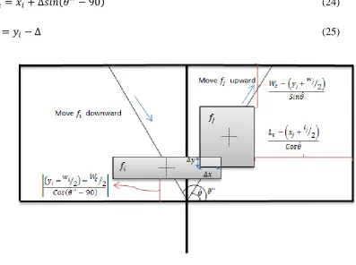
4.2. Repair Functions ... 45
4.2.1. General Steps of Repair Function ... 45
4.3. General Special Cases of Repair Function ... 47
4.3.1. Facility 𝑓𝑖 and facility 𝑓𝑗 in quadrant 𝑄1 ... 47
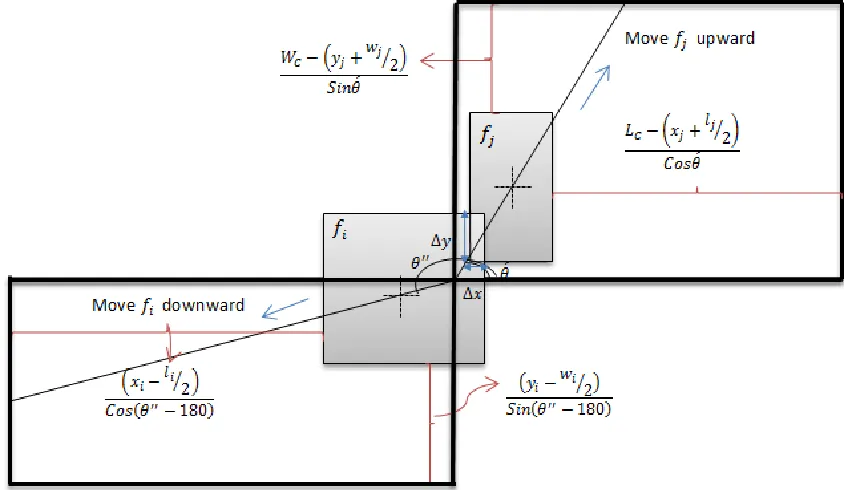
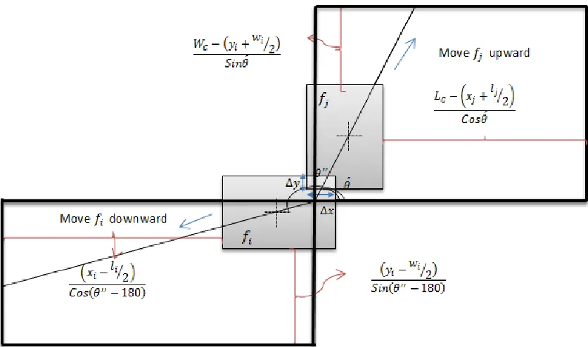
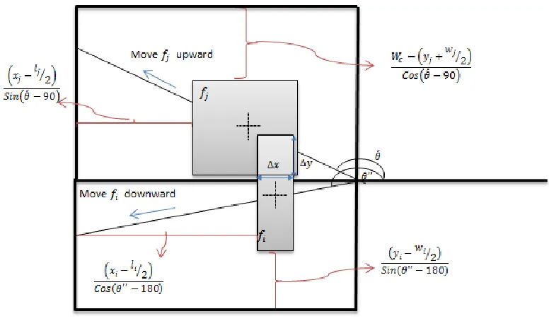
4.3.2. Facility 𝑓𝑖 in quadrant 𝑄2 ... 53
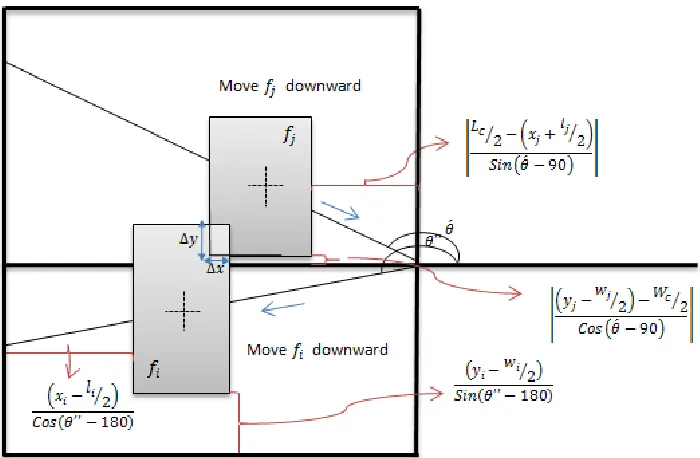
4.3.3. Facility 𝑓𝑖 in quadrant 𝑄3 ... 63
4.3.4. Facility 𝑓𝑖 in quadrant 𝑄4 ... 72
4.4. Improved Heuristic ... 83
4.5. Metaheuristic Algorithm ... 85
4.5.1. Simulated Annealing ... 85
4.5.2. Why not using greedy algorithms? ... 85
4.5.3. SA Procedures ... 86
4.5.4 The elements of SA algorithm ... 86
4.5.5. The General Pseudo Code of SA ... 90
4.5.6. Developed Simulated Annealing for FLP ... 93
4.5.7. Developed SA Algorithm ... 106
4.5.8. Improved Repair Function ... 107
CHAPTER FIVE: CASE STUDY ... 113
5.1. Company Description ... 113
5.1.1. Products and Machine Tools ... 113
5.1.2. Shop Floor ... 114
x
5.2. Computational Results ... 117
5.2.1. Mathematical Modelling ... 117
5.2.2. Heuristics ... 128
5.2.3. Validation of SA ... 140
CHAPTER SIX: CONCLUSION ... 156
References ... 158
Appendices ... 162
xi
LIST OF TABLES
Table (1): FLP Discrete approach versus. FLP continuous approach ... 3
Table (2): Literature review summaries ... 16
Table (3): Length of vector 𝑟⃗⃗⃗ 𝑓, radial movement ... 38
Table (4): Calculation of coordinates of target facility ... 39
Table (5): The distance left between facility fi and the boundaries of site ... 42
Table (6): New coordinate of 𝑓𝑖 after applying repair function ... 82
Table (7): Length of vectors 𝑟⃗⃗⃗ 1 and 𝑟⃗⃗⃗ 2 ... 83
Table (8): SA parameters ... 89
Table (9): 𝐶 and 𝐶́ coordinates ... 96
Table (10): New coordinate of 𝑓𝐺 after move ... 97
Table (11): Revised coordinate based on Before-Aisle repair function- horizontal aisle ... 103
Table (12): Revised coordinate based on Before-Aisle repair function -vertical aisle ... 103
Table (13): Revised coordinate based on After-Aisle repair function -horizontal aisle ... 109
Table (14): Revised coordinate based on After-Aisle repair function - vertical aisle ... 109
Table (15). Machine tools descriptions ... 114
Table (16). Parts’ specifications and the operations sequence ... 115
Table (17). GF results ... 116
Table (18): Intra-cell layout for Primary Cell- Nonlinear model ... 118
Table (19): Intra-cell layout for Grinding Cell- Nonlinear model ... 119
Table(20): Intra-cell layout for Diamond Cell- Nonlinear model ... 120
Table(21): Intra-cell layout for Final Cell- Nonlinear model ... 121
Table (22): Inter-cell layout - Nonlinear model ... 122
Table (23): Intra-cell layout for Primary Cell- linear model ... 123
xii
Table (25): Intra-cell layout for Diamond Cell- Linear model ... 125
Table(26): Intra-cell layout for Final Cell- Linear model ... 126
Table (27): Inter-cell layout-Linear model ... 127
Table (28): Intra-cell layout for Primary Cell- Heuristic algorithm ... 128
Table (29): Intra-cell layout for Grinding Cell- Heuristic algorithm ... 129
Table (30): Intra-cell layout for Diamond Cell- Heuristic algorithm ... 130
Table (31): Intra-cell layout for Final Cell- Heuristic model ... 131
Table (32): Initial solution-Primary Cell ... 132
Table (33): Initial solution-Grinding Cell ... 132
Table (34): Initial solution-Diamond Cell ... 132
Table (35): Initial solution-Final Cell ... 133
Table (36): Intra-cell layout for primary Cell- SA algorithm ... 134
Table (37): Intra-cell layout for grinding Cell- SA algorithm ... 135
Table (38): Intra-cell layout for diamond Cell- SA algorithm ... 136
Table (39): Intra-cell layout for final Cell- SA algorithm ... 137
Table (40): Inter-cell initial solution for SA algorithm ... 138
Table (41): Inter-cellular layout based on SA algorithm ... 139
Table (42): 1st run of SA algorithm for Primary Cell ... 140
Table (43): 2nd run of SA algorithm for Primary Cell ... 140
Table (44): 3rd run of SA algorithm for Primary Cell ... 140
Table (45): 4th run of SA algorithm for Primary Cell ... 141
Table (46): 5th run of SA algorithm for Primary Cell ... 141
Table (47): 6th run of SA algorithm for Primary Cell ... 141
Table (48): 7th run of SA algorithm for Primary Cell ... 141
Table (49): 8th run of SA algorithm for Primary Cell ... 142
Table (50): 9th run of SA algorithm for Primary Cell ... 142
Table (51): 10th run of SA algorithm for Primary Cell ... 142
Table (52): 1rd run of SA algorithm for Grinding Cell ... 143
Table (53): 2th run of SA algorithm for Grinding Cell ... 143
Table (54): 3th run of SA algorithm for Grinding Cell ... 143
xiii
Table (56): 5th run of SA algorithm for Grinding Cell ... 144
Table (57): 6th run of SA algorithm for Grinding Cell ... 144
Table (58): 7th run of SA algorithm for Grinding Cell ... 144
Table (59): 8th run of SA algorithm for Grinding Cell ... 144
Table (60): 9th run of SA algorithm for Grinding Cell ... 144
Table (61): 10th run of SA algorithm for Grinding Cell ... 145
Table (62): 1st run of SA algorithm for Diamond Cell ... 146
Table (63): 2nd run of SA algorithm for Diamond Cell ... 146
Table (64): 3rd run of SA algorithm for Diamond Cell ... 146
Table(65): 4th run of SA algorithm for Diamond Cell ... 146
Table (66): 5th run of SA algorithm for Diamond Cell ... 147
Table (67): 6th run of SA algorithm for Diamond Cell ... 147
Table (68): 7th run of SA algorithm for Diamond Cell ... 147
Table (69): 8th run of SA algorithm for Diamond Cell ... 147
Table (70): 9th run of SA algorithm for Diamond Cell ... 148
Table (71): 11th run of SA algorithm for Diamond Cell ... 148
Table (72): 1st run of SA algorithm for Final Cell ... 149
Table (73): 2nd run of SA algorithm for Final Cell ... 149
Table (74): 3rd run of SA algorithm for Final Cell ... 149
Table (75): 4th run of SA algorithm for Final Cell ... 149
Table (76): 5th run of SA algorithm for Final Cell ... 149
Table (77): 6th run of SA algorithm for Final Cell ... 150
Table (78): 7th run of SA algorithm for Final Cell ... 150
Table (79): 8th run of SA algorithm for Final Cell ... 150
Table (80): 9th run of SA algorithm for Final Cell ... 150
Table (81): 10th run of SA algorithm for Final Cell ... 150
Table (82): 1st run of SA algorithm for Inter-cellular layout ... 151
Table (83): 2nd run of SA algorithm for Inter-cellular layout ... 151
Table (84): 3rd run of SA algorithm for Inter-cellular layout ... 151
Table (85): 4th run of SA algorithm for Inter-cellular layout ... 151
xiv
Table (87): 6th run of SA algorithm for Inter-cellular layout ... 152
Table (88): 7th run of SA algorithm for Inter-cellular layout ... 152
Table (89): 8th run of SA algorithm for Inter-cellular layout ... 152
Table (90): 9th run of SA algorithm for Inter-cellular layout ... 153
Table (91): 10th run of SA algorithm for Inter-cellular layout ... 153
Table (92): Comparisons between mathematical modeling and simulate annealing... 154
xv
LIST OF FIGURES
Figure (1): Scheme of facilities regard to their corresponding cell ... 23
Figure (2): The Scheme of cells regard to the shop ... 25
Figure (3): The scheme of shop ... 26
Figure (4): Scheme of block constraints ... 33
Figure (5): The scheme of radial movement ……… 37
Figure (6): Scheme of overlap between two facilities ……… 40
Figure (7): Facility 𝑓𝑖 and facility 𝑓𝑗 in quadrant 𝑄1, 𝑦𝑖 ≥ 𝑦𝑗, 𝑥𝑖 ≤ 𝑥𝑗, ∆𝑥 ≥∆𝑦 .... 48
Figure (8): Facility 𝑓𝑖 and facility 𝑓𝑗 in quadrant 𝑄1, 𝑦𝑖 ≥ 𝑦𝑗, 𝑥𝑖 ≤ 𝑥𝑗, ∆𝑥 ≤∆𝑦 .... 49
Figure (9): Facility 𝑓𝑖 and facility 𝑓𝑗 in quadrant 𝑄1, 𝑦𝑖 ≥ 𝑦𝑗, 𝑥𝑖 ≥ 𝑥𝑗, ∆𝑥 ≥∆𝑦 .... 50
Figure (10): Facility 𝑓𝑖 and facility 𝑓𝑗 in quadrant 𝑄1, 𝑦𝑖 ≥ 𝑦𝑗, 𝑥𝑖 ≥ 𝑥𝑗, ∆𝑥 ≤∆𝑦 ... 50
Figure (11): Facility 𝑓𝑖 and facility 𝑓𝑗 in quadrant 𝑄1, 𝑦𝑖 ≤ 𝑦𝑗, 𝑥𝑖 ≤ 𝑥𝑗, ∆𝑥 ≤∆𝑦 ... 51
Figure (12): Facility 𝑓𝑖 and facility 𝑓𝑗 in quadrant 𝑄1, 𝑦𝑖 ≤ 𝑦𝑗, 𝑥𝑖 ≤ 𝑥𝑗, ∆𝑥 ≥∆𝑦 ... 52
Figure (13): Facility 𝑓𝑖 in quadrant 𝑄2 and facility 𝑓𝑗 in quadrant 𝑄1, 𝑦𝑖 ≤ 𝑦𝑗, , ∆𝑥 ≤∆𝑦 ... 54
Figure (14): Facility 𝑓𝑖 in quadrant 𝑄2 and facility 𝑓𝑗 in quadrant 𝑄1, 𝑦𝑖 ≤ 𝑦𝑗, , ∆𝑥 ≥∆𝑦 ... 55
Figure (15): Facility 𝑓𝑖 in quadrant 𝑄2 and facility 𝑓𝑗 in quadrant 𝑄1, 𝑦𝑖 ≥ 𝑦𝑗, , ∆𝑥 ≤∆𝑦 ... 56
Figure (16): Facility 𝑓𝑖 in quadrant 𝑄2 and facility 𝑓𝑗 in quadrant 𝑄1, 𝑦𝑖 ≥ 𝑦𝑗, , ∆𝑥 >∆𝑦 ... 58
Figure (17): Facility 𝑓𝑖 and facility 𝑓𝑗 in quadrant 𝑄2, 𝑦𝑖 ≥ 𝑦𝑗, 𝑥𝑖 ≤ 𝑥𝑗, ∆𝑥 ≤∆𝑦 .. 59
Figure (18): Facility 𝑓𝑖 and facility 𝑓𝑗 in quadrant 𝑄2, 𝑦𝑖 ≥ 𝑦𝑗, 𝑥𝑖 ≤ 𝑥𝑗, ∆𝑥 >∆𝑦 .. 59
Figure (19): Facility 𝑓𝑖 and facility 𝑓𝑗 in quadrant 𝑄2, 𝑦𝑖 < 𝑦𝑗, 𝑥𝑖 ≤ 𝑥𝑗, ∆𝑥 >∆𝑦 .. 60
Figure (20): Facility 𝑓𝑖 and facility 𝑓𝑗 in quadrant 𝑄2, 𝑦𝑖 < 𝑦𝑗, 𝑥𝑖 ≤ 𝑥𝑗, ∆𝑥 ≤∆𝑦 .. 61
Figure (21): Facility 𝑓𝑖 and facility 𝑓𝑗 in quadrant 𝑄2, 𝑦𝑖 < 𝑦𝑗, 𝑥𝑖 ≥ 𝑥𝑗, ∆𝑥 >∆𝑦 .. 62
Figure (22): Facility 𝑓𝑖 and facility 𝑓𝑗 in quadrant 𝑄2, 𝑦𝑖 < 𝑦𝑗, 𝑥𝑖 ≥ 𝑥𝑗, ∆𝑥 ≤∆𝑦 .. 62
xvi
Figure (24): Facility 𝑓𝑖 in quadrant 𝑄3 and facility 𝑓𝑗 in quadrant 𝑄1, ∆𝑥 >∆𝑦 .... 64
Figure (25): Facility 𝑓𝑖 in quadrant 𝑄3 and facility 𝑓𝑗 in quadrant 𝑄2, 𝑥𝑖 ≤ 𝑥𝑗, ∆𝑥 ≤ ∆𝑦 ... 65
Figure (26): Facility 𝑓𝑖 in quadrant 𝑄3 and facility 𝑓𝑗 in quadrant 𝑄2, 𝑥𝑖 ≤ 𝑥𝑗, ∆𝑥 ≥ ∆𝑦 ... 66
Figure (27): Facility 𝑓𝑖 in quadrant 𝑄3 and facility 𝑓𝑗 in quadrant 𝑄2, 𝑥𝑖 ≥ 𝑥𝑗, ∆𝑥 ≥ ∆𝑦 ... 66
Figure (28): Facility 𝑓𝑖 in quadrant 𝑄3 and facility 𝑓𝑗 in quadrant 𝑄2, 𝑥𝑖 ≤ 𝑥𝑗, ∆𝑥 ≤ ∆𝑦 ... 67
Figure (29): Facility 𝑓𝑖 and facility 𝑓𝑗 in quadrant 𝑄3, 𝑦𝑖 ≥ 𝑦, 𝑥𝑖 ≥ 𝑥𝑗, ∆𝑥 ≤∆𝑦 ... 68
Figure (30): Facility 𝑓𝑖 and facility 𝑓𝑗 in quadrant 𝑄3, 𝑦𝑖 ≥ 𝑦, 𝑥𝑖 ≥ 𝑥𝑗, ∆𝑥 ≥∆𝑦 ... 68
Figure (31): Facility 𝑓𝑖 and facility 𝑓𝑗 in quadrant 𝑄3, 𝑦𝑖 ≤ 𝑦𝑗, 𝑥𝑖 ≤ 𝑥𝑗, ∆𝑥 ≥∆𝑦.. 69
Figure (32): Facility 𝑓𝑖 and facility 𝑓𝑗 in quadrant 𝑄3, 𝑦𝑖 ≤ 𝑦𝑗, 𝑥𝑖 ≥ 𝑥𝑗, ∆𝑥 ≥∆𝑦.. 70
Figure (33): Facility 𝑓𝑖 and facility 𝑓𝑗 in quadrant 𝑄3, 𝑦𝑖 ≤ 𝑦𝑗, 𝑥𝑖 ≤ 𝑥𝑗, ∆𝑥 >∆𝑦.. 71
Figure (34): Facility 𝑓𝑖 in quadrant 𝑄4and facility 𝑓𝑗 in quadrant 𝑄1, 𝑥𝑖 ≥ 𝑥𝑗, ∆𝑥 ≥∆𝑦 ... 72
Figure (35): Facility 𝑓𝑖 in quadrant 𝑄4and facility 𝑓𝑗 in quadrant 𝑄2, 𝑥𝑖 ≥ 𝑥𝑗, ∆𝑥 ≥∆𝑦 ... 73
Figure (36): Facility 𝑓𝑖 in quadrant 𝑄4and facility 𝑓𝑗 in quadrant 𝑄3, 𝑦𝑖 ≥ 𝑦𝑗, ∆𝑥 ≤∆𝑦 ... 74
Figure (37): Facility 𝑓𝑖 in quadrant 𝑄4and facility 𝑓𝑗 in quadrant 𝑄3, 𝑦𝑖 ≥ 𝑦𝑗, ∆𝑥 ≥∆𝑦 ... 75
Figure (38): Facility 𝑓𝑖 in quadrant 𝑄4and facility 𝑓𝑗 in quadrant 𝑄3, 𝑦𝑖 ≤ 𝑦𝑗, ∆𝑥 ≥∆𝑦 ... 76
Figure (39): Facility 𝑓𝑖 in quadrant 𝑄4and 𝑓𝑗 in quadrant 𝑄3 , 𝑦𝑖 ≤ 𝑦𝑗, ∆𝑥 ≤∆𝑦 ... 77
Figure (40): Facility 𝑓𝑖 and facility 𝑓𝑗 in quadrant 𝑄4, 𝑦𝑖 ≤ 𝑦𝑗, ∆𝑥 ≤∆𝑦 ... 78
Figure (41): Facility 𝑓𝑖 and facility 𝑓𝑗 in quadrant 𝑄4, 𝑦𝑖 ≤ 𝑦𝑗, ∆𝑥 ≥∆𝑦 ... 78
Figure (42): Facility 𝑓𝑖 and facility 𝑓𝑗 in quadrant 𝑄4, 𝑦𝑖 ≥ 𝑦𝑗, 𝑥𝑖 ≥ 𝑥𝑗, ∆𝑥 ≥∆𝑦 ... 79
xvii
Figure (44): Facility 𝑓𝑖 and facility 𝑓𝑗 in quadrant 𝑄4, 𝑦𝑖 ≥ 𝑦𝑗, 𝑥𝑖 ≤ 𝑥𝑗, ∆𝑥 ≥∆𝑦 ... 81
Figure (45): Heuristic v.s. Greedy algorithm ... 86
Figure (46): Flowchart of Simulated Annealing ... 92
Figure (47): Angle calculation in move operator (I) ... 95
Figure (48): Concept of Angle in move operator (II) ... 96
Figure (49): Free zone concept ... 99
Figure (50): Before-Move operator for horizontal aisle ... 104
Figure (51): Before-Aisle-Move operator for vertical aisle ... 105
Figure (52): After-Aisle-Operator for horizontal aisle ... 110
Figure (53): After-Aisle-Operator for vertical aisle ... 111
Figure (54): Scheme of company’s shop floor ... 114
Figure (55): Intra-cell layout of Primary Cell- Nonlinear Model ... 118
Figure (56): Intra-cell layout of Grinding Cell- Nonlinear Model ... 119
Figure (57): Intra-cell layout for Diamond Cell- Nonlinear Model ... 120
Figure (58): Intra-cell layout for Final Cell- Nonlinear Model ... 121
Figure (59): Inter-cell layout design- Nonlinear Model ... 122
Figure (60): Intra-cell layout of Primary cell- Linear Model ... 123
Figure (61): Intra-cell layout of Grinding cell- Linear Model ... 124
Figure (62): Intra-cell layout of Diamond cell- Linear Model ... 125
Figure (63): Intra-cell layout of Diamond cell- Linear Model ... 126
Figure (64): Inter-cell layout design-Linear Model ... 127
Figure (65): Primary Cell Layout Based on Developed Heuristic ... 128
Figure (66): Grinding Cell Layout Based on Developed Heuristic ... 129
Figure (67): Diamond Cell Layout Based on Developed Heuristic ... 130
Figure (68): Final Cell Layout Based on Developed Heuristic ... 131
Figure (69): Primary Cell Layout Based on SA ... 134
Figure (70): Grinding Cell Layout Based on SA ... 135
Figure (71): Diamond Cell Layout Based on SA ... 136
Figure (72): Final Cell Layout Based on SA ... 137
Figure (73): Initial solution for inter-cell layout using heuristic ... 138
xviii
LIST OF APPENDECIES
APPENDIX ONE: MOVE OPERATOR ………...……… 162
APPENDIX TWO: SWAP OPERATOR ………... 167
APPENDIX THREE: OVERLAP CHECKING FUNCTION …...……… 172
APPENDIX FOUR: SA ALGORITHM …………...……… 175
APPENDIX FIVE: HEURISITC ………...……… 181
xix
LIST OF
ACRONYMS
MIP Mixed Integer Programming
NLMIP NonLinear Mixed Integer Programming
QAP Quadratic Assignment Program
FLP Facility Layout Problem
DFLP Dynamic Facility Layout Problem CMS Cellular Manufacturing System
CM Cellular Manufacturing
GF Group Formation
CL Cell Layout
GT Group Technology
GS Group Scheduling
MHC Material Handling Cost
UA-FLP Unequal sized Facility Layout Problem
SA Simulate Annealing
GA Genetic Algorithm
xx
NOMENCLATURE
List of Nomenclature- Nonlinear Mixed Integer Model
𝑃 = {1,2,3, … , 𝑃} Index set of part types 𝑀 = {1,2,3, … , 𝑀} Index set of machine types 𝐶 = {1,2,3, … , 𝐶} Index set of cell types
𝑂𝑝 = {1,2,3, … , 𝑂𝑝} Index set of operations indices for part p
L Horizontal dimension of shop floor
W vertical dimension of shop floor
𝑌𝑉𝐴𝐿𝑈 Vertical dimension of upper side of aisle 𝑌𝑉𝐴𝐿𝐿 Vertical dimension of lower side of aisle
𝑋𝐻𝐴𝐿𝐿𝐹 Horizontal dimension of left side of aisle 𝑋𝐻𝐴𝐿𝑅𝑇 Horizontal dimension of right side of aisle
𝑙𝑖 Length of machine i
𝑤𝑖 Width of machine i
𝑙́𝑐 Length of cell c
𝑤́𝑐 Width of cell c
𝐶𝐴𝑗 Intracellular transfer unit cost for part j
𝐶𝐸𝑗 Intercellular transfer unit cost for part j
xxi
𝑈𝑗𝑜𝑖 1, if operation o of part j is done by machine i, otherwise 0
𝑈𝑗𝑜𝑐́ 1, if operation o of part j is done by machine i which is located in cell c,
otherwise 0
𝑄𝑖𝑐 1, if machine i is assigned in cell c
𝑥𝑖 Horizontal distance between center of machine i and vertical reference line
𝑦𝑖 Vertical distance between center of machine i and horizontal reference line 𝑥𝑐 Horizontal distance between center of cell c and vertical reference line 𝑦𝑐 Vertical distance between center of cell c and horizontal reference line
𝑍𝑖𝑢 1, if machine u is arranged in the same horizontal level as machine i, and 0 otherwise
𝑊𝑐𝑐́ 1, if cell 𝑐 is arranged in the same horizontal level as cell 𝑐́ and 0 otherwise
𝑍𝑐 1, if cell 𝑐 is arranged in out of horizontal aisle boundaries and 0 otherwise
𝑊𝑐 1, if cell 𝑐 is arranged in out of vertical aisle boundaries and 0 otherwise
List of Nomenclature- Linear Model
𝑄𝑋𝑖𝑢 1, if horizontal dimension of facility 𝑖 is greater than horizontal dimension
of facility 𝑢
𝑄𝑌𝑖𝑢 1, if vertical dimension of facility 𝑖 is greater than vertical dimension of facility 𝑢
𝑄𝑋𝑐𝑐́ 1, if horizontal dimension of cell 𝑐 is greater than horizontal dimension of cell 𝑐́
xxii List of Nomenclature- Block Constraints
K Number of blocks
𝑥𝑏𝑙𝑜𝑐𝑘𝑘 The horizontal coordinate of block k
𝑦𝑏𝑙𝑜𝑐𝑘𝑘 The vertical coordinate of block k
𝑙𝑏𝑙𝑜𝑐𝑘𝑘 The length of block k
𝑤𝑏𝑙𝑜𝑐𝑘𝑘 The width of block k
1
CHAPTER ONE: INTRODUCTION
1.1.Background
In this thesis, the facility layout problem (FLP) for particular class of manufacturing systems, where is cellular manufacturing system (CMS) has been tackled. In this section; the background and physics of the different elements pertaining to the problem at hand are explained. We start by explaining what is CMS; that is to be followed by definition of FLP and finally, some synopsis of the overall approach taken has been provided.
1.1.1. Cellular Manufacturing System
Cellular manufacturing system (CMS) layout has recently begun to receive heightened attention worldwide. Cellular Manufacturing (CM) is an application of GTCM is the combination of job shop and/or flow shop. In CM the site is divided physically into small groups which each are dedicated to parts which have similarities in process and operations requirement, machinery. The groups are called cells and the similar parts are named as part families. Generally speaking, each cell is designed to produce a part family. However, in the real world converting to pure CMS is impossible. Usually there are some parts that cannot be categorized in unique part family. Hence, the whole production process cannot be finished in one cell. Furthermore, there are some machine tools used as general utilization, these kinds of machine tools cannot be placed in specific cell. These kinds of parts and machine tools are placing in specific cells called reminder cell. There are some machine tools which cannot be assigned in specialized cell or reminder cell because of safety or economic issues such as those machine tools which produce too much heat that have to be placed in specific area of shop (Green & Sadowski, 1984).
2
production, and (4) resource allocation – assigning tools and human and materials resources.
An effective CMS implementation help any company improve machine utilization and quality; it also makes reduction in setup time, work-in-process inventory, material handling cost, part makespan, and expediting costs (Wemmerlov & Johnson, 1997; Ariafar et al., 2011; Defersha and Chen, 2006).
1.1.2. Facility Layout Problem
3 1.1.3. Approach
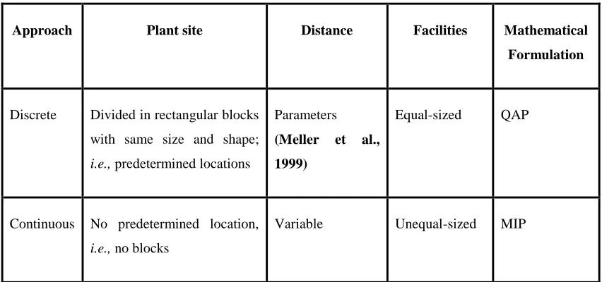
Several algorithms have been developed for FLP problem. Traditional approach to FLP problem called discrete representation often addressed by quadratic assignment problem (QAP) with the objective of minimizing a given function cost. There are two main assumptions in QAP: firstly all facilities are equal size and shape; secondly the locations of facilities are known in a priori. However these kinds of assumptions are not applicable in real world case studies. This approach to FLP is not suited to represent the exact locations of facilities; and cannot formulate FLP especially when facilities are unequal size and shape or if there are different clearances between the facilities. The more proper approach to such kind of cases is continuous representation rather than discrete. There are two ways to solve this problem. Chronologically, the first one attempts at dividing each facility into smaller size unit blocks, where the total area of those blocks is approximately equal to the area of the facility. There are two drawbacks to this method: firstly the problem size is growing as the total number of blocks increase, and secondly the exact shapes of facilities are ignored. The second approach to continuous problem assumes the exact shape and dimensions of the facilities.
Table (1): FLP Discrete approach versus. FLP continuous approach
Approach Plant site Distance Facilities Mathematical
Formulation
Discrete Divided in rectangular blocks
with same size and shape;
i.e., predetermined locations
Parameters
(Meller et al.,
1999)
Equal-sized QAP
Continuous No predetermined location,
i.e., no blocks
4 1.2.Motivation of thesis
FLP to CMS is focusing on the second step of design of CMS which by itself is two folds: inter-cell and intra-cell layout. The main objective of group layout is minimizing material handling cost (MHC) by arranging facilities in their corresponding cells and cells in floor. In this work, both demand and operation sequencing have been considered in optimizing the layout both at inter and intra cellular levels However, this was not the case with literature; there is a dearth of papers that happened to take a discrete approach which really did addressed those factors. Moreover, in this thesis we are adopting a continuous approach.
In this work, the detailed cellular layout problem has been addressed for both shop floor level and that at cellular level. In the literature, however for CMS significant of the work has solved only the block layout problem where layout problem at inter cellular was addressed.
The third motivation is taking more effective approach to FLP problem, i.e., taking continuous approach. From proper engineering and practical outlook there is no predetermined location for facilities. By assuming specific locations for facilities, the chance to get more effective layout design is being decreased. Because lots of facilities’ arrangements options are ignored. Moreover, by taking continuous approach the limitation of facilities’ size is relaxed. Hence, in the developed model there is no restriction to the size of the facilities.
Finally, since FLP is a NP-hard problem, developing heuristics algorithms is the other motivation of this thesis. Designing heuristics algorithm for discrete FLP is easier than continuous approach. Because, the only operator needs is swap operator,
5
problems are high which requires designing variety of repair function to eliminate overlap.
1.3.Outline of the thesis
6
CHAPTER TWO: LITERATURE REVIEW
2.1. Problem definition
The facility layout problem (FLP) for cellular manufacturing system (CMS) is considered in this thesis. By taking systematic manufacturing outlook to FLP, the problem is to arrange facilities that are cells in the leader problem and machine tools in the follower problem in the continual planar site. The physics of the problem is as follows: machine tools, cells, and shop have rectangular shape with specific length and width.
To determine the flow rate operations sequence and different part’s demand are considered. Each part compromises certain operations with specific sequence which is processed by dedicated machine tools. By predetermining group formation ahead of time; it has already known which machine belongs to which cell; and which operation of machine is processed in which cell; i.e., operations of part j processed in cell k are known ahead of time. Speaking about the material flows between facilities the traffic within a cell is the material flow among the machines located in cell, and at shop floor (factory) level material flows between cells are actually the flows among the operations of parts on machines done in each cell. Therefore, the objective function in both levels is minimizing material handling cost (MHC) which is 𝑓𝑙𝑜𝑤 × 𝑑𝑖𝑠𝑡𝑎𝑛𝑐𝑒.
2.2. Relevant Literature Review
Literature review has two main folds, in the first part previous paper done in quadratics assignment problem (QAP) problem- discrete approach is reviewed, and then mixed integer programming (MIP) problem- continuous approach toward FLP problem is considered.
2.2.1. Discrete Approach
7
metaheuristic algorithm for this kind of problem. Wilhelm and Ward (1987) apply simulated annealing (SA) to solve QAP. Their results have been compared with the Computerized Relative Allocation of Facilities Technique (CRAFT), biased sampling and revised Hillier problem and showed better quality solutions.
Baykasoglu and Gindy (2001) apply the SA for dynamic layout problem, discrete approach. They claim their proposed algorithm finds better solution. They compared their proposed algorithm to the three works done such as Rosenblatt (1986), Conway and Vekataramanan (1994), and Balakrishnan and Cheng (2000). In the first comparison, their SA approach found optimum solution and revealed better solution than dynamic programming algorithm of Rosenblatt (1986). The second comparison has two experiments; first one done with no shifting cost and the SA algorithm found optimum solution and outperforms that Conway and Vekataramanan (1994) genetic algorithm. In this experiment relocation costs are included. The optimum solution was not found, however the results of SA showed a slight improvement than outputs of Conway and Vekataramanan (1994). Finally, in third comparison the data set obtained from Balakrishnan and Cheng (2000). They develop nonlinear genetic algorithm (NLGA). The comparison between SA-based approach and NLGA reveals the superiority of SA algorithm when the size of the problems is large. Since they have taken discrete approach to FLP, the only operator has been used in neighbourhood generation algorithm is the swap operator.
Tavakolli-Moghaddam et al., (2005) develop a nonlinear mathematical modelling to solve the cell formation in dynamic environment in which demand varies in each time horizon. The strength point of their model is that it is a multi-objective model i.e.,
8
Defersha and Chen (2006) provide a comprehensive manufacturing attributes used in CF design. They develop a MIP multi-objective mathematical programming for cell formation problem. The proposed model tries to minimize machine maintenance and overhead cost, machine procurement cost, inter-cell travel cost, machine operation and setup cost, tool consumption cost, and system configuration cost. The model incorporates several factors such as dynamic cell configurations, alternative routings, lot splitting, sequence of operations, multiple processing, tool consumption cost, set up cost, cell size limits, and machine adjacency constraints. They provide some numerical examples for small size of problem. No heuristic algorithm has been presented in their work.
Wu et. al., (2006) propose a mathematical model to solve GF and GL (inter-cell and intra-cell) concurrently by minimizing total travel cost (inter and intra-cell) and the number of exceptional elements. They incorporate important factor such as part demand, machine capacity, operation sequence, transfer batch. Finally, a hierarchical genetic algorithm (HGA) is developed to solve the problem. In another study Wu et al., (2007a) propose a HGA form manufacturing cells and determine the group layout of a CMS concurrently. The novelty of their presented algorithm is a new hierarchical chromosome structure, a selection scheme, and a group mutation operator.
Tavakoli-Moghaddam et al., (2007) develop a nonlinear model for GF both inter-cell and intra-inter-cell movement. The special feature of their work is that they are considering stochastic demand. They assume equal sized machine tools and cells; also unrestricted shop floor. It means that there is no restriction on the shape and dimensions of the shop floor. In order to prove their model, they use numerical example and no heuristic model has been developed.
9
positive features such as considering all aspects of reconfiguration such as adding, removing and replacing machine tools. Moreover, maximum cell size and machine time capacity are the two main constraints considered in this model. These constraints make sense because it is not efficient to make one cell too crowed and the other one not as. Furthermore, machine capacity also is considered in this model. The other point is using operation sequence in calculating inter and intra material handling cost There are some drawbacks to the work as well. Firstly all machine tools assumed have equal size. Secondly, the other assumption is the equal distance between all cells and machine tools which is not happening in very realistic.
Airafar et al., (2011) present a mathematical formulation to for facility layout plan in a hybrid cellular manufacturing system and develop a SA algorithm to solve the model. The interesting point of their model is that the demand varies during planning horizon. However, like as other QAP models they assume the equal size of facilities which is not applicable in real world cases. The other drawback to their model is that the shape and size of the shop floor is unrestricted, while it is not happen in any real case studies. In another study Airafar et al., (2012) investigate the effect of demand variation on arrangement of facilities i.e. the demand has normal distribution. They develop a stochastic nonlinear integer programming by these assumptions that all facilities are equal sized, and there is no restriction on shape and dimension of shop floor. These two assumptions are the main limitations of the proposed model. No heuristic developed for solving the proposed model and the model solved by numerical examples.
10
total costs of intra and inter-cell material handling, machine relocation, purchasing new machines, machine overhead and machine processing. This study by looking at discrete approach to layout design is one of the comprehensive models. Finally they develop a SA algorithm to solve the model.
Recently, some efforts have been done to integrate all three aspects of CMS such as GF, GL and GS. Wu et al., (2007b) propose a model to integrate the CF, GL and GS decisions concurrently. The objective function is minimizing the makespan. The model is solved by a hierarchical genetic algorithm. However their mathematical formulation is not clear enough. Firstly, they defined “machine position number index” and calculated the distance between two machines by subtracting the corresponding position numbers. The question here is that how they calculate the exact distance between machines and cells. The second critique to their work is that, they have not considered parts’ demand or material movements among machines. They try to integrate the three main aspects of CMS just based on minimizing makespan. However, in reality there are several factors affecting CMS such as parts demand, inter-cell and intra-cell material movement that has to be considered. Third, their proposed model is static, so the dynamicity in the product mix and demand is not considered in their model. Finally, they have taken discrete approach to CMS design which means predetermined locations for machines, that by itself is a poor assumption.
2.2.2. Continuous Approach- MIP
The first MIP for FLP has been presented by Montreuil (1990). Herague and Kusiak (1991) develop the special case of Montreuli’s model which the length, width, and orientation of facilities known in advance. They represent two models; one linear continuous and the second one linear mixed integer. They develop a heuristic method-penalty method to solve their models.
11
SA has been used to find the initial solution, and then a heuristic approach based on penalty model developed to improve the solution. The main limitation of this model is that the cell locations are predetermined.
12
decision makers the chance to consider how changing preferences’ priorities would impact the solutions.
The other important piece of research was written by Imam and Mir (1993) and Mir and Imam (2001). Imam and Mir (1993) introduce a heuristic algorithm to place unequal sized rectangular facilities in continuous plane by introducing the new concept of “controlled coverage” by using “envelop blocks”. In the initial solution facilities are randomly placed in plane in the envelop block the size of which is much larger than the actual size of facility and is calculated by multiplying magnification factor with the facilities’ actual dimensions. Afterwards, during the heuristic iterations the sizes of envelop blocks are gradually decreased by decreasing the magnification factor until the dimensions of envelopes till became equal to the dimensions of their corresponding facilities. By this approach they were controlling the coverage of facilities together. The improvement iteration is based on the univariate search method. In this method only one of the 2𝑛 design variables which 𝑛 is the number of facilities is changing at time. This change means moving facility horizontally or vertically along X-axis or Y-axis respectively. There are three draw backs to their method. Firstly, each iteration cycle is repeated 2𝑛 times, 𝑛 times to move facilities horizontaly and then another 𝑛 more times to move them vertically. The other drawback is that facilities are just allowed to move horizontally or vertically, there is no diagonal movement. Thirdly, there are no borders for the assumed continuous plane. However, in real world there is no plane without borders. The last drawback is related to magnification factor, they have not specified how large this factor has to be originally and by which fraction it has to be reduced in each iteration cycle.
13
factor is equal to one. So it is obvious that the computational cost and time is quite dependent of magnification factor.
Tain et. al., (2010) develop a mixed integer linear programming (MILP) to solve dynamic facility layout plan; i.e., layout plan is not fixed for all period of time. They develop a GA to solve their model. Their work is quite unique. Once, the model is considering dynamicity to the FLP. Additionally, the rearrangement cost also is applied beside cost of material flow. They define rearrangement as changes in facility’s coordinates or orientation. Finally, the budget constraint assumed for rearrangement cost. This approach has one drawback which is distracting the continuance aspect of their assumed FLP, because this method forces facilities to be placed within specific lines.
There are recent studies that have adopted a continuous approach (Arkat et al.,
2012 a, b). In the first study Arkat et al., (2012 a)define two nonlinear mixed integer mathematical models. The first model developed to integrate cell formation problem with cell layout both inter-cell and intra-cell with the objective of minimizing total transportation cost of parts. The second model proposed to concurrently solve the formation of cells, cellular layout and cellular scheduling by minimising makespan. They develop a GA algorithm to solve the model. In the second study, Arkat et al.,
(2012 b) present a multi-objectives mathematical modelling to solve CF, CL, and CS simultaneously. The two objectives are minimizing both total transportation cost and makespan cost. A multi-objective genetic algorithm (MOGA) is then developed to solve the problem. Using sequence of operation as well as considering non-overlap elimination constraints are the two strength points of their studies. However, there are two main drawbacks to their both models as are explaining below:
14
overlap between the two machines. Note that ∆x and ∆y are the difference in 𝑥 and 𝑦 coordinates between the centroids of the two machines named respectively. However, still this does not really rule out all possible scenarios where one would have overlap.
2) The constraints formulated do not really rule out the possibility of having non-rectangular cells as being claimed.
3) The constraints used to force machines to stay within shop floor boundaries are also not accurate. Since the 𝑥𝑖 and 𝑦𝑖 are centroid dimensions of each machine and we assume the length (ℎ𝑖) and width (𝑣𝑖) of machine i, hence end corner points for length
of each machine would be 𝑥𝑖 −ℎ𝑖
2 and 𝑥𝑖 + ℎ𝑖
2 and the same for width 𝑦𝑖− 𝑣𝑖
2 and
𝑦𝑖+𝑣2𝑖 . Therefore, if we assume W and L is vertical and horizontal distance of shop
floor respectively, the boundary constraints would be 𝑥𝑖 +ℎ2𝑖≥ 𝐿, 0 ≤ 𝑥𝑖−ℎ2𝑖 for length and 𝑦𝑖−𝑣2𝑖 ≥ 0 and 𝑦𝑖+𝑣2𝑖≤ 𝑊 for width of shop floor.
4) Arkat et al.,(2012) have assumed that the machines have equal square area and cells are rectangle. However, in the real world these are poor assumptions.
2.3. Gap Analysis
Table (2) summarizes our findings and provides a comprehensive gap analysis. It is observed that FLP can be solved either by discrete approach or continuous approach. Discrete approach is the popular one because of its simplicity. The main assumptions considered in discrete approach are equal sized facilities, predetermined locations, and unrestricted shop. However, those are poor assumptions in the real world. Therefore, there is a need to develop a solution for FLP by assuming more realistic assumptions such as unequal sized facilities, restricted shop and no predetermined locations.
15
design of layout plan have not been considered in literature extensively. Aisle structures, fixed facilities’ positions and fixed department are considered in this work. The problem has been considered in this thesis have manufacturing focus which is FLP toward cellular layout problem. Hence, considering manufacturing attributes such as operations’ sequence and part demand are so important. This was addressed by Kia et al., (2012); however the approach taken is discrete approach. Bazargan-Lari and Kaebernick (1997) have developed a comprehensive mathematical modeling and hybrid model for CMS. However they have not considered operation sequence in their studies. Mir and Imam (2001) also have developed a hybrid model for FLP; however firstly they do not take a manufacturing outlook into the problem. Hence, their approach is just placing facilities in continual plane site. Finally, Arkat et al.,(2012 a,b) has not applied part demands and moreover, all facilities assumed have unit square shape. Placing equal sized facilities are easier than unequal sized facilities.
23
CHAPTER THREE: MATHEMATICAL MODELING
At the core of the approach being taken, the group layout (GL) problem for CMS has been modeled and solved sequentially in steps. Group formation has been assumed to done a priori. A two-tier mixed integer non-linear programming model has been developed to solve the intra-cell and inter-cell layout sequentially at two different hierarchical levels, namely at the cellular and shop floor levels. The details are declared as follows.
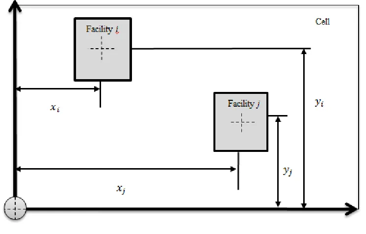
3.1. Leader Problem- Intra-cell Layout
Since the Group Formation is done in advance, it is already known which machine is assigned to which cell. In this level the layout of group of facilities in their corresponding cell is being designed. Hence, the leader problem is the layout at the cell. The centroid of the facility is the reference for the coordinates of that facility. It has to be noted the origin for facilities’ coordinates is their left bottom corner of their relative cell. Figure (1) represents the scheme of facilities regard to their corresponding cell.
24
It is important to note that initially when running the FLP for each cell (leader problem), an upper limits for the length and width of each cell are being defined by using constraints named as within-cell constraint. In other words, by assumption 𝑙𝑐and 𝑤𝑐 as the length and width of cell c, the summation of the centroid horizontal dimension of each facility ( 𝑥𝑖 ) and the half of length of that facility has to be less than equal to the length of the cell, and similarly the centroidal vertical dimensions of each facility ( 𝑦𝑖 ) and the half of width of that facility has to be less than or equal to the width of the cell. Moreover, at leader level, the traffic at intra-level is the material flow among the machines (operations already assigned to machines) located in cell, the position of which the intercellular layout problem is yet to be determined.
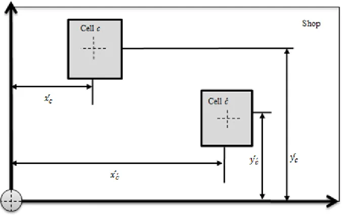
3.2. Follower Problem- Inter-cell Layout
After the layout for all manufacturing cells have been finalized, the overall approach for the whole which is follower problem is being solved. Thus, follower is the layout for the whole shop (i.e. intercellular). The coordinates of cells are calculated based on the horizontal and vertical distance of the centroid of the cell to the origin of the whole shop which is left bottom corner of the shop. Similarly, the within constraints are applied in the follower problem as well. To illustrate, the cells have to be located within the boundaries of the whole shop. In other words, if shop has length
25
Figure (2): The scheme of cells regard to the shop
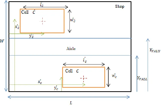
3.3 Problem Statement
26
Figure (3): Scheme of shop
The problem is formulated under the following assumptions: 1. CF is known in advanced.
2. Machines are not in the same size.
3. Machines must be located within a given area. 4. Machines are not allowed overlap to each other. 5. Cell’s dimensions and orientation are predetermined.
6. Each part type has a number of operations that must be processed based on its operation sequence readily available from the route sheet of parts. It should be noted that the process sequence of each parts are different.
7. The demand for each part type in known and is constant
8. Material handling devices moving the one part between machines.
9. Inter and intra-cell movements related to the part types have different costs is related to the distance traveled. We assume that the rectangular distance between each pair of machines’ centroid.
27
3.4. NonLinear Mixed Integer Programming Model (NLMIP)
The mathematical formulation represented as below:
Sets:
𝑃 = {1,2,3, … , 𝑃} Index set of part types 𝑀 = {1,2,3, … , 𝑀} Index set of machine types 𝐶 = {1,2,3, … , 𝐶} Index set of cell types
𝑂𝑝 = {1,2,3, … , 𝑂𝑝} Index set of operations indices for part p
Parameters:
L Horizontal dimension of shop floor
W vertical dimension of shop floor
𝑌𝑉𝐴𝐿𝑈 Vertical dimension of upper side of aisle
𝑌𝑉𝐴𝐿𝐿 Vertical dimension of lower side of aisle 𝑋𝐻𝐴𝐿𝐿𝐹 Horizontal dimension of left side of aisle
𝑋𝐻𝐴𝐿𝑅𝑇 Horizontal dimension of right side of aisle
𝑙𝑖 Length of machine i
𝑤𝑖 Width of machine i
𝑙𝑐 Length of cell c
𝑤𝑐 Width of cell c
𝐶𝐴𝑗 Intracellular transfer unit cost for part j
28 𝐷𝑗 Demand quantity for part j
𝑈𝑗𝑜𝑖 1, if operation o of part j is done by machine i, otherwise 0
𝑈𝑗𝑜𝑐́ 1, if operation o of part j is done by machine i which is located in cell c,
otherwise 0
𝑄𝑖𝑐 1, if machine i is assigned in cell c
Decision variables:
𝑥𝑖 Horizontal distance between center of machine i and vertical reference line
𝑦𝑖 Vertical distance between center of machine i and horizontal reference line 𝑥𝑐́ Horizontal distance between center of cell c and vertical reference line 𝑦𝑐́ Vertical distance between center of cell c and horizontal reference line
𝑍𝑖𝑢 1, if machine u is arranged in the same horizontal level as machine i, and 0 otherwise
𝑊𝑐𝑐́ 1, if cell 𝑐 is arranged in the same horizontal level as cell 𝑐́ and 0 otherwise
𝑍𝑐 1, if cell 𝑐 is arranged in out of aisle horizontal boundaries and 0 otherwise 𝑊𝑐 1, if cell 𝑐 is arranged in out of aisle vertical boundaries and 0 otherwise
The continuous bi-level programming problem is defined as: The intra-cell layout mathematical formulation to layout the different machines (machines here are the facilities) of every cell c at a time is as follows:
Min ∑ ∑ ∑𝑀𝑖,𝑢=1𝑈𝑗𝑜𝑖 𝑈𝑗𝑜+1𝑢(|𝑥𝑖− 𝑥𝑢| + |𝑦𝑖− 𝑦𝑢|) 𝐶𝐴𝑗𝐷𝑗
𝑖≠𝑢 𝑜𝑝−1
𝑜=1 𝑃
𝑗=1 (1)
29 𝑥𝑖+𝑙𝑖
2 ≤ 𝑙𝐶 𝑖 = 1, . . , 𝑀 (2)
𝑥𝑖−𝑙2𝑖 ≥ 0 𝑖 = 1, . . , 𝑀 (3)
𝑦𝑖 +𝑤2𝑖 ≤ 𝑤𝑐 𝑖 = 1, . . , 𝑀 (4)
𝑦𝑖 −𝑤2𝑖 ≥ 0 𝑖 = 1, . . , 𝑀 (5)
|𝑥𝑖 − 𝑥𝑢| ≥ 𝑍𝑖𝑢(𝑙𝑖+ 𝑙𝑢)/2 𝑖, 𝑢 = 1, . . , 𝑀 (6) |𝑦𝑖− 𝑦𝑢| ≥ (1 − 𝑍𝑖𝑢)(𝑤𝑖 + 𝑤𝑢)/2 𝑖, 𝑢 = 1, . . , 𝑀 (7)
𝑥𝑖, 𝑦𝑖 ≥ 0, 𝑍𝑖𝑢 are binary 𝑖, 𝑢 = 1, . . , 𝑀 (8)
Equation 1 declares the objective function of leader problem which is minimizes the total intra-cell transportation cost of parts. Equations 2 to 5 are within-site constraints that ensure each machine tool are assigned within the boundaries of its corresponding cell. Equations 6 and 7 force the overlap elimination for machine tools. Equation 8 represents the nature of the decision variables which are binary and non-negative.
Finally, the inter-cell layout problem tries to layout the different cells (cells here are the facilities) of the entire shop floor is as follows:
Min ∑ ∑ ∑𝐶𝑐,𝑐́=1𝑈𝑗𝑜𝑐́ 𝑈𝑗𝑜+1𝑐́́ (|𝑥𝑐́ − 𝑥𝑐́́ | + |𝑦𝑐́ − 𝑦𝑐́́ |) 𝑐≠𝑐́
𝑜𝑝−1
𝑜=1 𝑃
𝑗=1 𝐶𝐸𝑗𝐷𝑗 (9)
s.t
𝑥𝑐́ +𝑙𝑐 ́
2 ≤ 𝐿 𝑐 = 1, . . , 𝐶 (10)
𝑥𝑐́ −𝑙𝑐 ́
30
𝑦𝑐́ +𝑤2𝑐́ ≤ 𝑊 𝑐 = 1, . . , 𝐶 (12)
𝑦𝑐́ −𝑤2𝑐́ ≥ 0 𝑐 = 1, . . , 𝐶 (13)
|𝑥𝑐́ − 𝑥𝑐́́ | ≥ 𝑊𝑐𝑐́(𝑙́ + 𝑙𝑐 𝑐́́ )/2 𝑐, 𝑐́ = 1, . . , 𝐶 (14)
|𝑦𝑐́ − 𝑦𝑐́́ | ≥ (1 − 𝑊𝑐𝑐́)(𝑤𝑐́ + 𝑤́ )/2𝑐́ 𝑐, 𝑐́ = 1, . . , 𝐶 (15)
Aisle Constraints:
Horizontal Aisle:
(𝑦𝑐́ + 𝑤́ /2) − 𝑌𝑐 𝑉𝐴𝐿𝐿≤ M 𝑍𝑐 (16)
𝑌𝑉𝐴𝐿𝑈− (𝑦𝑐́ − 𝑤𝑐́ /2) ≤ M (1 − 𝑍𝑐) (17)
Vertical Aisle:
(𝑥𝑐́ − 𝑙́ /2) − 𝑋𝑐 𝐻𝐴𝐿𝑅𝑇 ≤ 𝑀𝑊𝑐 (18)
𝑋𝐻𝐴𝐿𝐿𝐹− (𝑥𝑐́ + 𝑙́ /2) ≤ 𝑀(1 − 𝑊𝑐 𝑐) (19)
𝑥𝑐́ , 𝑦𝑐́ ≥ 0, 𝑊𝑐𝑐́ , 𝑍𝑐 , 𝑊𝑐 are binary 𝑐 = 1, . . , 𝐶 (20)
31 3.5. Linearization
Since both overlap eliminations constraints and objective functions have absolute terms, two terms are using for linealization.
3.5.1. Linearization of Objective Function
In order to linearize the absolute terms of leader problem’s objective function, the linearized variables defined is such a term to satisfy equations (21) and (22).
|𝑥𝑖 − 𝑥𝑢| = 𝑥𝑖𝑢+ − 𝑥𝑖𝑢− (21)
|𝑦𝑖− 𝑦𝑢| = 𝑦𝑖𝑢+ − 𝑦𝑖𝑢− (22)
The two above terms (21) and (22) are replaced by absolute terms in the objective function (equation 1). Moreover, those equations (21) and (22) are added to the constraints. Hence, the linearized objective function of leader problem would be:
Min ∑ ∑ ∑𝑀𝑖,𝑢=1𝑈𝑗𝑜𝑖 𝑈𝑗𝑜+1𝑢((𝑥𝑖𝑢+ − 𝑥𝑖𝑢− ) + (𝑦𝑖𝑢+ − 𝑦𝑖𝑢−)) 𝐶𝐴𝑗𝐷𝑗 𝑖≠𝑢
𝑜𝑝−1
𝑜=1 𝑃
𝑗=1 (23)
Similarly; for linearizing follower problem’s objective function (9) the new linearized variables defined which have to satisfied equations (24) and (25). These constraints are replaced in the nonlinear objective function:
|𝑥𝑐́ − 𝑥𝑐́́ | = 𝑥𝑐𝑐́́ − 𝑥+
𝑐𝑐́−́ (24)
|𝑦𝑐́ − 𝑦𝑐́́ | = 𝑦𝑐𝑐́́ − 𝑦+ 𝑐𝑐́−́ (25)
Hence the linearized objective function of follower problem is:
Min ∑ ∑ ∑𝐶𝑐,𝑐́=1𝑈𝑗𝑜𝑐́ 𝑈𝑗𝑜+1𝑐́́ ((𝑥𝑐𝑐́́ − 𝑥+ 𝑐𝑐́−́ ) + (𝑦𝑐𝑐́́ − 𝑦+ 𝑐𝑐́−́ )) 𝑐≠𝑐́
𝑜𝑝−1
𝑜=1 𝑃
32 3.5.2. Linearization of Constraints
The overlap elimination constraints of leader and follower problems (6)-(7) and (14)-(15) respectively have absolute terms which declare the nonlinearity nature of those constraints. In order to linearize, two variables are introduced:
Moreover, the following constraints substitute by constraints (6) and (7)
(𝑥𝑖− 𝑥𝑢) + 𝑀 × 𝑄𝑋𝑖𝑢 ≥ 𝑍𝑖𝑢(𝑙𝑖 + 𝑙𝑢)/2 𝑖, 𝑢 = 1, . . , 𝑀 (27)
(𝑥𝑖− 𝑥𝑢) − 𝑀 × (1 − 𝑄𝑋𝑖𝑢) ≤ (−𝑍𝑖𝑢)(𝑙𝑖 + 𝑙𝑢)/2 𝑖, 𝑢 = 1, . . , 𝑀 (28)
(𝑦𝑖− 𝑦𝑢) + 𝑀 × 𝑄𝑌𝑖𝑢 ≥ (1 − 𝑍𝑖𝑢)(𝑤𝑖 + 𝑤𝑢)/2 𝑖, 𝑢 = 1, . . , 𝑀 (29) (𝑦𝑖− 𝑦𝑢) − 𝑀 × (1 − 𝑄𝑌𝑖𝑢) ≤ −(1 − 𝑍𝑖𝑢)(𝑤𝑖+ 𝑤𝑢)/2 𝑖, 𝑢 = 1, . . , 𝑀 (30)
Similarly; Furthermore, the four following constraints are replaced by constraints (14) and (15) in non-linear inter-cell problem:
(𝑥𝑐́ − 𝑥𝑐́́ ) + 𝑀 × 𝑄𝑋𝑐𝑐́ ≥ 𝑊𝑐𝑐́(𝑙́ + 𝑙𝑐 𝑐́́ )/2 𝑐, 𝑐́ = 1, . . , 𝐶 (31)
(𝑥𝑐́ − 𝑥𝑐́́ ) − 𝑀 × (1 − 𝑄𝑋𝑐𝑐́) ≤ (−𝑊𝑐𝑐́)(𝑙́ + 𝑙𝑐 ́ )/2𝑐́ 𝑐, 𝑐́ = 1, . . , 𝐶 (32)
(𝑦𝑐́ − 𝑦𝑐́́ ) + 𝑀 × 𝑄𝑌𝑐𝑐́ ≥ (1 − 𝑊𝑐𝑐́)(𝑤𝑐́ + 𝑤́ )/2𝑐́ 𝑐, 𝑐́ = 1, . . , 𝐶 (33)
(𝑦𝑐́ − 𝑦𝑐́́ ) − 𝑀 × (1 − 𝑄𝑌𝑐𝑐́) ≤ −(1 − 𝑊𝑐𝑐́)(𝑤𝑐́ + 𝑤́ )/2 𝑐, 𝑐́ = 1, . . , 𝐶𝑐́ (34)
33 3.6. The Blocks Constraints
In some situations, some specific areas cannot be occupied by facilities such as inventory area. Moreover, in some certain conditions the locations of some facilities are fixed and cannot be changed based on the economic reasons or safety and so on. In these cases those areas or facilities are assumed as blocks with the exact length and width as well as coordinates. The figure (4) shows the scheme of block constraints.
Figure (4): the scheme of block constraints
In order to consider those constraints, the below constraints are added NLMIP of follower problem:
|𝑥𝑐́ − 𝑥𝑏𝑙𝑜𝑐𝑘𝑘| ≥ 𝑍𝑐𝑘́ (𝑙́ + 𝑙𝑏𝑙𝑜𝑐𝑘𝑐 𝑘)/2 𝑐 = 1, . . , 𝐶,𝑘 = 1, . . , 𝐾 (35)
|𝑦𝑐́ − 𝑦𝑏𝑙𝑜𝑐𝑘𝑘| ≥ (1 − 𝑍𝑐𝑘́ )(𝑤𝑐́ + 𝑤𝑏𝑙𝑜𝑐𝑘𝑘)/2 𝑐 = 1, . . , 𝐶, 𝑘 = 1, . . , 𝐾 (36)
Which:
K Number of blocks
𝑥𝑏𝑙𝑜𝑐𝑘𝑘 The horizontal coordinate of block k
34 𝑙𝑏𝑙𝑜𝑐𝑘𝑘 The length of block k
𝑤𝑏𝑙𝑜𝑐𝑘𝑘 The width of block k
𝑍𝑐𝑘́ 1 if cell 𝑐 is arranged in the same horizontal level as block 𝑘, and 0 otherwise
Constraints (35) and (36) prevent overlap between the blocks and cells.
There are absolute terms in the constraints (35) and (36), in order to linearize these constraints, the following four constraints substitute with constraints (35) and (36) by defining two binary variables called 𝑋𝐵𝑐𝑘 and 𝑌𝐵𝑐𝑘.
(𝑥𝑐́ − 𝑥𝑏𝑙𝑜𝑐𝑘𝑘) + 𝑀𝑋𝐵𝑐𝑘 ≥ 𝑍𝑐𝑢́ (𝑙𝑐́ + 𝑙𝑏𝑙𝑜𝑐𝑘𝑘)/2 𝑐 = 1, . . , 𝐶, 𝑘 = 1, . . , 𝐾
(37)
(𝑥𝑐́ − 𝑥𝑏𝑙𝑜𝑐𝑘𝑘) − 𝑀 × (1 − 𝑋𝐵𝑐𝑘) ≤ (−𝑍́ )(𝑙𝑐𝑢 𝑐́+ 𝑙𝑏𝑙𝑜𝑐𝑘𝑘)/2 𝑐 = 1, . . , 𝐶, 𝑘 =
1, . . , 𝐾 (38)
(𝑦𝑐́ − 𝑦𝑏𝑙𝑜𝑐𝑘𝑘) + 𝑀 × 𝑌𝐵𝑐𝑘 ≥ (1 − 𝑍𝑐𝑢́ )(𝑤́ + 𝑤𝑏𝑙𝑜𝑐𝑘𝑐 𝑘)/2𝑐 = 1, . . , 𝐶, 𝑘 = 1, . . , 𝐾
(39)
(𝑦𝑐́ − 𝑦𝑏𝑙𝑜𝑐𝑘𝑘) − 𝑀 × (1 − 𝑌𝐵𝑐𝑘) ≤ −(1 − 𝑍𝑐𝑢́ )(𝑤𝑐́ + 𝑤𝑏𝑙𝑜𝑐𝑘𝑘)/2𝑐 = 1, . . , 𝐶, 𝑘 = 1, . . , 𝐾
35 3.7. Limitation of Study
36
CHAPTER FOUR: HEURISTICS
4.1. Heuristic
In order to develop the feasible and efficient initial solution for the developed metaheuristic algorithm-simulated annealing- a novel heuristic algorithm has been developed. The major idea behind the developed heuristic algorithm is to minimize the possibility of overlaps between facilities by imposing distance between the centroid of the two consecutive facilities. To do this facilities are scattered in the site by taking radial movement. Figure (5) represents the scheme of radial movement. To illustrate, facilities are placed in the site along a radial at specific angle. As explained in order to make distance between the facilities a specific angle 𝜃 is defined and applied between the centroid of the two neighbor facilities. The angle 𝜃 is calculated by dividing 360𝑜 over the total number of facilities. Hence, 𝜃 = 3600
𝑀 . To start the heuristic algorithm,
at first all facilities are placed on top of each other in the middle of the site which is divided into four equal size quadrants i.e 𝑄1, 𝑄2, 𝑄3, 𝑄4. The heuristic algorithm has compromised into two loops.
4.1.1. Outer Loop
In each iteration, one random facility called facility 𝑓𝐺 is chosen as a target facility and placed within the site by taking radial movement. In other words, facility 𝑓𝐺 is placed along the specific radius by taking the certain angle of the radial movement, called 𝜃́. The radius is the vector 𝑟⃗⃗⃗ 𝑓 with the origin of the centroid of the site and the
end of the boundary of the corresponding quadrant in which the facility 𝑓𝐺 is being placed. Furthermore, the angle 𝜃́ is calculated as:
37
Figure (5): The scheme of radial movement
Facility, 𝑓𝐺, is placed by end of vector 𝑎 , which is a vector of random magnitude along vector’s 𝑟⃗⃗⃗ 𝑓 direction. It has to be noted, the length of vector 𝑎 is a random number
between [0, |𝑟⃗⃗⃗ | − 𝑟]𝑓 , 𝑟 is the length of the diagonal of facility 𝑓𝐺. By this approach facility 𝑓𝐺 is placed within the site. Table (3) and table (4) represent the calculation of length of vector 𝑟⃗⃗⃗ 𝑓 and the coordinates of 𝑓𝐺 respectively.