Static-Memory-Hard Functions, and Modeling the Cost of Space vs. Time

(1)

Static-Memory-Hard Functions,

and Modeling the Cost of Space vs. Time

Thaddeus Dryja Quanquan C. Liu Sunoo Park MIT

Abstract

A series of recent research starting with (Alwen and Serbinenko, STOC 2015) has deepened our understanding of the notion ofmemory-hardnessin cryptography — a useful property of hash functions for deterring large-scale password-cracking attacks — and has shown memory-hardness to have intricate connections with the theory of graph pebbling. Definitions of memory-hardness are not yet unified in the somewhat nascent field of memory-hardness, however, and the guarantees proven to date are with respect to a range of proposed definitions. In this paper, we observe two significant and practical considerations that are not analyzed by existing models of memory-hardness, and propose new models to capture them, accompanied by constructions based on new hard-to-pebble graphs. Our contribution is two-fold, as follows.

First, existing measures of memory-hardness only account for dynamic memory usage (i.e., memory read/written at runtime), and do not considerstatic memory usage (e.g., memory on disk). Among other things, this means that memory requirements considered by prior models are inherently upper-bounded by a hash function’s runtime; in contrast, counting static memory would potentially allow quantification of much larger memory requirements, decoupled from runtime. We propose a new definition ofstatic-memory-hard function (SHF) which takes static memory into account: we model static memory usage by oracle access to a large preprocessed string, which may be considered part of the hash function description. Static memory requirements are complementary to dynamic memory requirements: neither can replace the other, and to deter large-scale password-cracking attacks, a hash function will benefit from beingboth dynamic-memory-hard and static-dynamic-memory-hard. We give two SHF constructions based on pebbling. To prove static-memory-hardness, we define a new pebble game (“black-magic pebble game”), and new graph constructions with optimal complexity under our proposed measure. Moreover, we provide a prototype implementation of our first SHF construction (which is based on pebbling of a simple “cylinder” graph), providing an initial demonstration of practical feasibility for a limited range of parameter settings.

Secondly, existing memory-hardness models implicitly assume that the cost of space and time are more or less on par: they consider onlylinear ratios between the costs of time and space. We propose a new model to capturenonlinear time-space trade-offs: e.g., how is the adversary impacted when space is quadratically more expensive than time? We prove that nonlinear tradeoffs can in fact cause adversaries to employ different strategies from linear tradeoffs.

(2)

1 Introduction

Pebble games were originally formulated to model time-space tradeoffs by a game played on DAGs. Generally, a DAG can be thought to represent a computation graph where each node is associated with some computation and a pebble placed on a node represents saving the result of its computation in memory. Thus, the number of pebbles represents the amount of memory necessary to perform some set of computations. The natural complexity measures to optimize in this game is the minimum number of pebbles used, as well as the minimum amount of time it takes to finish pebbling all the nodes; these goals correspond with minimizing the amount of memory and time of computation.

Pebble games were first introduced to study programming languages and compiler construc-tion [PH70] but have since then been used to study a much broader range of tasks such as register allocation [Set75], proof complexity [AdRNV17, Nor12], time-space tradeoffs in Turing machine computation [Coo73, HPV77], reversible computation [Ben89], circuit complexity [Pot17], and time-space tradeoffs in various algorithms such as FFT [Tom81], linear recursion [Cha73, SS79b], matrix multiplication [Tom81], and integer multiplication [SS79a] in the RAM as well as the external memory model [JWK81]. To see a more comprehensive survey of the results in pebbling up to the last couple of years, see [Pip82] up to the 1980s and [Nor15] up to 2015.

The relationship between pebbling and cryptography has been a subject of research interest for decades, which has enjoyed renewed activity in the last few years. A series of recent works [AB16, ABH17, ABP17a, ABP17b, AS15, AT17, ACP+16, AAC+17, BZ16, BZ17] has deepened our understanding of the notion ofmemory-hardness in cryptography, and has shown memory-hardness to have intricate connections with the theory of graph pebbling.

Memory-hard functions (MHFs) have garnered substantial recent interest as a security measure against adversaries trying to perform attacks at scale, particularly in the ubiquitous context of password hashing. Consider the following scenario: hashes of user passwords are stored in a database,1 and when a user enters a password p to log in, her computer sendsH(p) to the database server, and the server compares the received hash to its stored hash for that user’s account. For a normal user, it would be no problem if hash evaluation were to take, say, one second. An attacker trying to guess the password by brute-force search, on the other hand, would try orders of magnitude more passwords, so a one-second hash evaluation could be prohibitively expensive for the attacker.

The evolution of password hashing functions has been something of an arms race for decades, starting with the ability to increase the number of rounds in the DES-based unix cryptfunction to increase its computation time—a feature that was used for exactly the above purpose of deterring large-scale password-cracking. Attackers responded by building special-purpose circuits for more efficient evaluation of crypt, resulting in a gap between the evaluation cost for an attacker and the cost for an honest user.2

A promising approach to mitigating this asymmetry in cost between hash evaluation on general-and special-purpose hardware is to increase the use ofmemory in the password hashing function. Memory is implemented in standardized ways which have been highly optimized, and memory chips are widely regarded to be an interchangeable commodity. Commonly used forms of memory — whether on-die SRAM cache, DRAM, or hard disks — are already optimized for the purpose of data I/O operations; and while there is active research in improving memory access times and costs, progress is and has been relatively incremental. This state of affairs sets up a relatively “even playing field,” as the normal user and the attacker are likely to be using memory chips of similar memory access speed. While an attacker may choose to buy more memory, the cost of doing so scales linearly with the amount purchased.

1_{In practice, the password should first be concatenated with a random user-specific string called a}_salt_{, and then} hashed. The salt is stored in the database alongside the hash to deterdictionary attacks.

2

(4)

The designs of several MHFs proposed to date (e.g., [Per09, AS15, AB16, ACP+16, ABP17a]) have proven memory-hardness guarantees by basing their hash function constructions on DAGs, and using space complexity bounds from graph pebbling. Definitions of memory-hardness are not yet unified in this somewhat nascent field, however — the first MHF candidate was proposed only in 2009 [Per09] — and the guarantees proven are with respect to a range of definitions. The “cumulative complexity”-based definitions of [AS15] have enjoyed notable popularity, but some of their shortcomings have been pointed out by subsequent work proposing alternative more expressive measures, in particular, [ABP17b, AT17].

Our contributionWe observetwo significant and practical considerations not analyzed by existing models of memory-hardness, and propose new models to capture them, accompanied by constructions based on new hard-to-pebble graphs. Our main contribution is two-fold, as described in (1) and (2) below. We also provide an additional contribution of separate interest, described in (3).

1. Static-memory-hardness. Existing measures of memory-hardness only account fordynamic

memory usage (i.e., memory read/written at runtime), and do not considerstatic memory usage (e.g., memory on disk). Among other things, this means that memory requirements considered by prior models are inherently upper-bounded by a hash function’s runtime; in contrast, counting static memory would potentially allow quantification of much larger memory requirements, decoupled from the honest evaluator’s runtime.

We propose a new definition of static-memory-hard function (SHF) (Definition 4.2), and present two SHF constructions based on pebbling. To prove static-memory-hardness, we define a new pebble game called theblack-magic pebble game (Definition 2.2), and prove properties of the space complexity of this game for new graphs (Graph Constructions 5.4 and 5.15). Graph Construction 5.15 gives rise to an SHF with a better asymptotic guarantee (same space usage but sustained over more time), whereas Graph Construction 5.4 yields an SHF with the advantage of simplicity in practice. Informal theorems stating the constructions’ static-memory-hardness guarantees are given in Section 1.3 and formal theorems are in Section 5. In Section 7, we discuss our prototype implementation based on Graph Construction 5.4.

We emphasize that static memory requirements are complementary to dynamic memory require-ments: neither can replace the other, and to deter large-scale password-cracking attacks, a hash function will benefit from being both dynamic-memory-hard and static-memory-hard.

2. Modeling nonlinear cost of space vs. time. Existing measures of memory-hardness

implicitly assume a linear trade-off between the costs of space and time. This model precludes situations where the relative costs of space and time might be more unbalanced (e.g., quadratic or cubic). We demonstrate that this modeling limitation is significant, by giving an example where adversaries facing asymptotically different space-time cost tradeoffs would in fact employ

different strategies. Then, to remedy this shortcoming, we define graph-optimal variants of memory-hardness measures (in Section 2) that explicitly model the relative cost of space and time. These can be seen as extending the main memory-hardness measures in the literature (namely, cumulative complexity and sustained memory complexity). We prove bounds on the

new measure as elaborated in Section 1.3.

3. We give the first graph construction that is tight, up to log logn-factors, to the optimal cumulative complexity that can be achieved for any graph (upper bound due to [ABP17a, ABP17b]).

Informal version of Theorem 6.23. There exists a family of graphs where the cumulative complexity of any constant in-degree graph withn nodes in the family is Θn2log log_log_n n which

(5)

Next, Section 1.1 gives a brief background on graph pebbling, Section 1.2 gives discussion on memory-hardness measures and related work, and Sections 1.3.1 and 1.3.4 give more detailed high-level overviews of our SHF contribution and nonlinear space-time tradeoff model (items (1) and (2) above), respectively.

1.1 Background on graph pebbling

The standard black pebble game is parametrized by a directed acyclic graph (DAG) and a special subset of its nodes (called thetarget set). In the game, an unlimited supply of “pebbles” is made available to a player, who must place and remove pebbles on the nodes of the DAG in a sequence of moves according to the following two rules.

1. A pebble may be placed or moved onto a node only if all of its predecessors have already been pebbled. (In particular, pebbles may be placed on source nodes at any time.)

2. Any pebble can be removed from the graph at any time.

The goal of the game is to arrive at a state where every pebble in the target set is covered by a pebble. Often, the target set is the set of the sink nodes.

The pebbling literature, starting with [PH70, Set75, Coo73, HPV77], has established a number of complexity measures describing the complexity of pebbling: e.g., measuring the minimum number of pebbles that must be used to achieve a complete pebbling, or the minimum number of moves needed. In the literature, there are several variants of the game, including sequential and parallel (depending on whether many pebbles can be placed in a single move), and versions where other different types of pebbles are used (such as the red-blue pebble game [JWK81] and the black-white pebble game [CS74]). In this work, our results are stated and proven in the context of constant in-degree graphs for simplicity; however, most of our results extend straightforwardly to non-constant in-degree graphs.

Graph pebbling and memory-hardness Graph pebbling algorithms can be used to construct hash functions in the (parallel) random oracle model. This paradigm has been used by prior constructions of memory-hard hashing [AS15] as well as other prior works [DKW11].

Informally, the idea to “convert” a graph into a hash function is to associate with each node v a string called alabel, which is defined to be O(v,pred(v)) whereO is a random oracle andpred(v) is the list of labels of predecessors of v. For source nodes, the label is instead defined to be O(v, ζ) for a string ζ which is an input to the hash function. The output of the hash function is defined to be the list of labels of target nodes. Intuitively, since the label of a node cannot be computed without the “random” labels of all its predecessors, any algorithm computing this hash function must move through the nodes of the graph according to rules very similar to those prescribed by the pebbling game; and therefore, the memory requirement of computing the hash function roughly corresponds to the pebble requirement of the graph. Thus, proving lower bounds on the pebbling complexity of graph families has useful implications for constructing provably memory-hard functions.

In our setting, in contrast to previous work, we employ a variant of the above technique: the string ζ is a fixed parameter of our hash function, and the input to the hash function instead specifies the indices of the target nodes whose labels are to be outputted.

1.2 Discussion on memory-hardness measures and related work

(6)

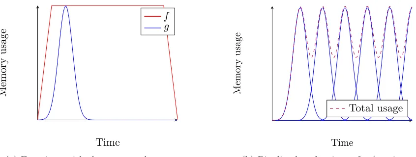
better for a password-cracking adversary. In particular, pipelining the evaluation of the latter type of function would allow reuse of the same memory for many function evaluations at once, effectively reducing the adversary’s amortized memory requirement by a factor of the number of concurrent executions (Figure 1b).

Fx

Time

Memory

usage

f g

(a) Functions with the same peak memory usage

Time

Memory

usage

Total usage

(b) Pipelined evaluations ofg(reusing memory) Figure 1: Limitations of peak memory usage as a memory-hardness measure

Cumulative complexity [AS15] put forward the notion ofcumulative complexity (CC), a com-plexity measure on graphs. CC was adopted by several subsequent works as a canonical measure of memory-hardness. CC measures the cumulative memory usage of a graph pebbling function evaluation: that is, the sum of memory usage over all time-steps of computation. In other words, this is the area under a graph of memory usage against time. CC is designed to be very robust against amortization, and in particular, scales linearly when computing many copies of a function on different inputs. This is a great advantage compared to the simpler measure of [Per09], which does not account well for an amortizing adversary (as shown in Figure 1).

Depth-robust graphs More recently, [AB16, ABP17a] proved bounds on optimal CC of certain graph families. They showed that a particular graph property calleddepth-robustness suffices to attain optimal CC (up to polylog factors–the CC of any graph with bounded in-degree is upper bounded byOn2log log_log_n n[AB16, ABP17b]). An (r, s)-depth-robust graph is one where there exists a path of lengthseven when any r vertices are removed. Intuitively, this captures the notion that storing anyr vertices of the graph will not shortcut the pebbling in a significant way. It turns out that depth-robustness will again be a useful property in our new model of memory-hardness with preprocessing.

(7)

Core-area memory ratio Previous works have considered certain hardware-dependent non-linearities in the ratio between the cost of memory and computation [BK15, AB16, RD17]. Such phenomena may incur a multiplicative factor increase in the memory cost that is dependent, in a possibly non-linear way, on specific hardware features. Note thatthe non-linearity here is in the hardware-dependence, rather than the space-time tradeoff itself. In contrast, our new models are more expressive, in that they make configurable the asymptotic tradeoff between space and time (by a parameter α which is in the exponent, as detailed in Definition 2.16) in an application-dependent way. This versatility of configuration targets applications where the trade-off may realistically depend on arbitrary and possibly exogenous space/time costs, and thus contrasts with metrics tailored for a specific hardware feature, such as core-memory ratio.

Towards a general theory of moderately hard functionsMost recently, Alwen and Tackmann [AT17] proposed a more general (though not comprehensive) framework for defining desirable guarantees of “moderately hard functions,” i.e., functions that are efficient to compute but somewhat hard to invert. Their work points out a number of drawbacks of prior measures such as those described above. Notably, many of the prior measures characterized the hardness of computing the function with an implicit assumption that this hardness would translate to the hardness ofinverting

the function (as it would indeed in the case of a brute-force approach to inversion). In other words, these measures implicitly assume that the hash function in question “behaves like a random oracle” in the sense that brute-force inversion is the optimal approach.

1.3 Our contributions in more detail

To prove static-memory-hardness, we define a new pebble game called the black-magic pebble game

(Definition 2.2), and prove properties of the space complexity of this game for new graphs (Graph Constructions 5.4 and 5.15).

The black-magic pebble game may additionally be of independent interest for the pebbling literature. Indeed, a pebble game used to analyze security of proofs of space [DFKP15] can be viewed as a non-adaptive3 version of the black-magic pebble game in which the target node set is sampled from a distribution by a challenger.

Based on our new graph constructions, we construct SHFs with provable guarantees on sustained memory usage, as follows. Graph Construction 5.15 gives a better asymptotic guarantee (same space usage but sustained over more time), whereas Graph Construction 5.4 has the advantage of simplicity in practice. In Section 7, we discuss our prototype implementation based on Graph Construction 5.4.

1.3.1 Static-memory-hard functions (SHFs)

Prior memory-hardness measures make a modeling assumption: namely, that the memory usage of interest is solely that of memory dynamically generated at run-time. However, static memory can be costly for the adversary too, and yet it is not taken into account by existing measures such as CC. Intuitively, it can be beneficial to design a function whose evaluation requires keeping a large amount of static memory on disk (which may be thought to be produced in a one-time initial setup phase). While not all the static memory might be accessed in any given evaluation, the “necessity” to maintain the data on disk can arise from the idea that an adversary attempting to evaluate the function on an arbitrary input while having stored a lesser amount of data would be forced to

dynamically generate comparable amounts of memory. Note that the resultingdynamic memory requirements could be orders of magnitude larger (say, gigabytes) than the memory requirements of

3

(8)

existing memory-hard function proposals, because unlike in prior memory-hardness models, here we have decoupled the memory requirement from the memory requirements of the honest evaluator.

We propose a new model and definitions for static-memory-hard functions (SHFs), in which we model static memory usage by oracle access to a large preprocessed string, which may be considered part of the hash function description. In particular, the preprocessed string can be public and known to the adversary — the important guarantee is that without storing (almost) all of it statically, the adversary will incur huge online memory requirements.

Definition (informal).We model a static-memory-hard function family as a two-part algorithm

H= (H₁,H₂) in the parallel random oracle model, whereH₁(1κ) outputs a “large” string to which

H₂ has oracle access,4 andH₂ receives an inputx and outputs a hash function outputy. Informally, our hardness requirement is that with high probability, anytwo-part adversary A= (A1,A2) must

either haveA1 output a large state (comparable to the output size of H1), or have A2 use large (dynamic) space.

We then give two constructions of SHFs based on graph pebbling. To prove static-memory-hardness, we define a new pebble game called the black-magic pebble game of which we give an overview in Section 1.3.3. Our simpler SHF construction is based on a family of tree-like “cylinder” graphs, which achieves memory usage proportional to the square root of the number of nodes, sustained over time proportional to the square root of the number of nodes. Furthermore, we give a better construction based on pebbling of a new graph family, that achieves better parameters: the same (square root) memory usage, but sustained over time proportional to the number of nodes.

Informal version of Theorem 5.28. The “cylinder graph” (Graph Construction 5.4) can be used to construct an SHF with static memory requirement Λ∈Θ(√n/(κ−ξlog(κ)) wherenis the number of nodes in the graph, κ is a security parameter, and ξ ∈ω(1), such that any adversary using non-trivially lessstatic memory than Λ must incur at least Λdynamic memory usage for at least Θ(√n) steps.

Informal version of Theorem 5.29. Graph Construction 5.15 can be used to construct an SHF with static memory requirement Λ∈Θ(√n)/(κ−ξlog(κ)) where n, κ, and ξare as described above, such that any adversary using non-trivially lessstaticmemory than Λ must incur at least Λdynamic

memory usage for at least Θ(n) steps.

Static memory requirements are complementary to dynamic memory requirements: neither can replace the other, and to deter large-scale password-cracking attacks, a hash function will benefit from beingboth dynamic-memory-hard and static-memory-hard. In Section 4.1, we give a discussion of how, given a static-memory-hard function and a (dynamic-)memory-hard function, they can be concatenated to yield a “dynamic SHF” that inherits both the static memory requirement of the former and the dynamic memory requirement of the latter.

Implementation We have a prototype implementation of our “cylinder” SHF construction. The code is available on github at https://github.com/adiabat/masshash. A discussion of the implementation and its performance for different static memory sizes is given in Section 7.

1.3.2 Remarks about the static-memory model

On static vs. dynamic memory In the case of function performing lookups to a large, static memory table, the memory storing the table does not need to be writable. This may seem to point to an optimization for the attacker: produce a read-only memory chip which supports fast, random-access read queries, but omits the hardware needed for writing data, as it has been pre-programmed

4

(9)

at the factory with the precomputed static table. However, in practice, this optimization seems implausible. In modern hardware, ROM chips have almost entirely disappeared; where they do still exist, they are used for their non-volatile storage properties (they retain data when power is lost, unlike most RAM), and are copied to RAM before being read from, due to the low speed of the ROM. Current development focuses almost exclusively on dynamic access memory which supports both reads and writes, so it is reasonable to believe that an attacker would need to use this type of hardware; switching to ROM would likely increase costs and slow down access to the static table.

Static and dynamic memory requirements are thus incomparable, and both are useful to deter a password-cracking adversary.

Alternative application: bounded retrieval (“big-key”) model As already stated above, the preprocessed string in our setting is assumed to be public, and our static-memory-hardness guarantees hold assuming the adversary knows the string. This is useful as it allows defining a single hash function accessible to all parties in a system, like a random oracle: one could imagine a standards body like NIST simply publishing a set of parameters defining a fixed hash function with a fixed “preprocessed string.” One informal way to think of this is that the preprocessed string is part of the description of a fixed hash function. A single hash function accessible to everyone is particularly useful for certain applications such as checksums, where many parties in a distributed network may need to compute the same hash function.

In some other applications, however, hash function families may suffice or be more appropriate, i.e., where each party samples a function from the family for her own use, rather than every party using exactly the same function. In such applications, the preprocessed string can be considered the seed of a particular hash function from the family defined by (H₁,H₂), and generated on a per-application basis. We observe one potential advantage of such a setup, inspired by the bounded retrieval [Dzi06, CLW06, CDD+07, ADW09, ADN+10, ADW09] (“big-key” [BKR16]) model.5: to make hash function evaluation more difficult for (e.g., password-cracking) adversaries. If the party using the hash function decides to keep the preprocessed string secret, then an adversary would have to exfiltrate almost all of the large preprocessed string from the honest user in order to be able to evaluate the hash function. As observed in the bounded retrieval literature, exfiltrating large quantities of data (say, gigabytes) can be much more costly for adversaries than exfiltrating smaller data items (such as secret keys).

1.3.3 Black-magic pebble game

We introduce a new pebble game called the black-magic pebble game. This game bears some similarity to the standard (black) pebble game, with the main difference that the player has access to an additional set of pebbles called magic pebbles. Magic pebbles are subject to different rules from standard pebbles: they may be placed anywhere at any time, but cannot be removed once placed, and may be limited in supply. The pebbling space cost of this game is defined as the maximum number of standard pebbles on the graph at any time-step plus the total number of magic pebbles used throughout the computation. Observe that while the most time-efficient strategy in the black-magic pebble game is always to pebble all the target nodes with magic pebbles in the first step, the most space-efficient strategy is much less clear.

Lower-bounds on space usage can be non-trivially different between the standard and magic pebbling games. For example, if a graph has a constant number of targets, then magic pebbling space usage will never exceed a constant number of pebbles, whereas the standard pebbling space usage can be super-constant. In particular, it is unclear, in the new setting of magic pebbling, whether

5

(10)

known lower-bounds on pebbling space usage in the standard pebble game6 are transferable to the magic pebble game. We prove in Section 5 that for layered graphs,7 the best possible lower-bound for the magic pebbling game is Θ(√n).

We leave determining the lower bound for magic pebbling space usage in general graphs as an open question. An answer to this open question would be useful towards constructing better static-memory-hard functions using the paradigm presented herein.

Our proof techniques rely on a close relationship between black-magic pebbling complexity and a new graph property which we define, called local hardness. Local hardness considers black-magic pebbling complexity in a variant model where subsets of target nodes are required to be pebbled (rather than all target nodes, as in the traditional pebbling game), and moreover, a “preprocessing phase” is allowed, wherein magic pebbles may be placed on the graph in advance of knowing which target nodes are to be produced. This “preprocessing” aspect bears some resemblance to the black-white pebbling game [CS74], a variant of the standard pebbling game in which some limited number of white pebbles can be placed “for free,” and the black pebbles must be placed according the standard rules. However, our setting differs from the black-white pebbling game: while preprocessing and storing magic pebbles in advance can be viewed as analogous to placing white pebbles for free, the black-white pebbling game imposes restrictions on theremoval of white pebbles from the graph, which are not present in our setting.

1.3.4 Capturing relative cost of memory vs. time

Existing measures such as CC and sustained memory complexity trade off space against time at a linear ratio. In particular, CC measures the minimal area under a graph of memory usage against time, over all possible algorithms that evaluate a function.8

However, different applications may have different relative cost of space and time. We propose and define a variant of CC called α-CC, parametrized byα which determines the relative cost of space and time, and observe thatα-CC may be meaningfully different from CC and more suitable for certain application scenarios. For example, when memory is “quadratically” more expensive than time, the measure of interest to an adversary may be the area under a graph of memory squared against time, as demonstrated by the following theorem.

Informal version of Theorem 6.8. There exist graphs for which an adversary facing a linear space-time cost trade-off would in fact employ adifferent pebbling strategy from one facing a cubic trade-off.

It follows that when the costs of space and time are not linearly related, the CC measure may be measuring the complexity ofthe wrong algorithm, i.e., not the algorithm that an adversary would in fact favor. We thus see that our α-CC measure is more appropriate in settings where space may be substantially more costly than time (or vice versa). Moreover, our parametrized approach generalizes naturally to sustained memory complexity. We show that our graph constructions are invariant across different values of α, a potentially desirable property for hash functions so that they are robust against different types of adversaries.

6

E.g., Θ n logn

space is necessary to pebble certain classes of graphs in the standard pebble game [LT82]. 7_{“Layered graph” is a standard term in the pebbling literature that refers to graphs whose nodes can be partitioned} into a sequence of “layers” such that edges only go between vertices in adjacent layers.

8

(11)

Informal version of Theorem 6.13. Given any graph constructionG= (V, E), there exists a pebbling strategy that is less expensive asymptotically than any strategy using a number of pebbles asymptotically equal to the number of nodes in the graph for any time-space tradeoff.

1.4 Organization of the rest of the paper

Section 2 introducesstandard and new graph pebbling definitions, Section 3 introduces computation in the parallel random oracle model and its relation to our newblack-magic pebbling complexity measures, Section 4 introduces our definition of a static-memory-hard function (SHF), Section 5 gives our SHF constructions and proofs. Then, Section 6 presents our modeling and motivation of nonlinear cost tradeoffs between space and time, with upper and lower bounds in the new model. Finally, Section 7 discusses our prototype SHF implementation.

2 Pebbling definitions

A pebbling game is a one-player game played on a DAG where the goal of the player is to place pebbles on a set of one or moretarget nodes in the DAG.

In Section 2.1, we formally define two variations of the sequential and parallel pebble games: the standard (black) pebble game and theblack-magic pebble game, the latter of which we introduce in this work. We also give the definitions of valid strategies and moves in these games. Then in Section 2.2, we define measures for evaluating the sequential and parallel pebbling complexity on families of graphs.

2.1 Standard and magic pebbling definitions

Definition 2.1 (Standard (black) pebble game).

• Input: A DAG, G= (V, E), and a target set T ⊆V. Define pred(v) = {u∈V : (u, v)∈E}, and let S⊆V be the set of sources of G.

• Rules at move i: At the start of the game, no node of G contains a pebble. The player has access to a supply of black pebbles. Game-play proceeds in discrete moves, and Pi (called a

“pebble configuration”) is defined as the set of nodes containing pebbles after theith move. P0=∅

represents the initial configuration where no pebbles have been placed. Each move may consist of multiple actions adhering to the following rules.9

1. A pebble can be placed on any source, s∈S. 2. A pebble can be removed from any vertex.

3. A pebble can be placed on a non-source vertex, v, if and only if its direct predecessors were pebbled at time i−1 (i.e., pred(v)∈Pi−1).

4. A pebble can be moved from vertexvto vertexwif and only if(v, w)∈E and pred(w)∈Pi−1.

• Goal: Pebble all nodes in T at least once (i.e.,T ⊆St

i=0Pi).10

Remark. At first glance, it may seem that rule 4 in Definition 2.1 is redundant as a similar effect can be achieved by a combination of the other rules. However, the application of rule 4 can allow the usage of fewer pebbles. For example, a simple two-layer binary tree (with three nodes) could

9

Multiple applications of rules 1, 2, and 3 can occur in a single move. E.g., multiple sources can be pebbled in a single move. Rule 4 can also be applied multiple times in a single movefor different pebbles, but cannot be applied more than once to the same pebble (since, naturally, a single pebble cannot move to multiple locations).

(12)

be pebbled with two pebbles using rule 4, but would require three pebbles otherwise. Nordstrom [Nor15] showed that in sequential strategies, it is always possible to use one fewer pebble by using rule 4.

We note for completeness that while rule 4 is standard in the pebbling literature, not all the papers in the MHF literature include rule 4.

Next, we define the black-magic pebble game which we will use to prove security properties of our static-memory-hard functions.

Definition 2.2 (Black-magic pebble game).

• Input: A DAG G= (V, E), a target set T ⊆V, and magic pebble bound M∈_N∪ {∞}.

• Rules: At the start of the game, no node of G contains a pebble. The player has access to two types of pebbles: black pebbles and up to M magic pebbles. Game-play proceeds in discrete moves, and Pi = (Mi, Bi) is the pebble configuration after the ith move, where Mi, Bi are the

sets of nodes containing magic and black pebbles after the ith move, respectively. P0 = (∅,∅)

represents the initial configuration where no black pebbles or magic pebbles have been placed. Each move may consist of multiple actions adhering to the following rules.

1. Black pebbles can be placed and removed according to the rules of the standard pebble game which are defined in the full version.11

2. A magic pebble can be placed on and removed from any node, subject to the constraint that at mostM magic pebbles are used throughout the game.

3. Each magic pebble can be placed at most once: after a magic pebble is removed from a node, it disappears and can never be used again.

• Goal: Pebble all nodes in T at least once (i.e.,T ⊆St

i=0(Mi∪Bi)).

Remark. In the black-magic pebble game, unlike in the standard pebble game, there is always the simple strategy of placing magic pebbles directly on all the target nodes. At first glance, this may seem to trivialize the black-magic game. When optimizing for space usage, however, this simple strategy may not be favorable for the player: by employing a different strategy, the player might be able to use much fewer thanT pebbles overall.

Next, we define valid sequential and parallel strategies in these games.

Definition 2.3(Pebbling strategy). LetGbe a graph andT be a target set. Astandard (resp., black-magic) pebbling strategy for (G, T)is defined as a sequence of pebble configurations,P ={P0, . . . , Pt},

satisfying conditions 1 and 2 below. P is moreover valid if it satisfies condition 3, and sequentialif it satisfies condition 4.

1. P0=∅.

2. For eachi∈[t],Pi can be obtained from Pi−1 by a legal move in the standard (resp., black-magic)

pebble game.

3. P successfully pebbles all targets, i.e.,T ⊆ St

i=0 Pi.

4. For each i∈[t], Pi contains at most one vertex not contained in Pi−1 (i.e., |Pi\Pi−1| ≤1).

A black-magic pebbling strategy must satisfy one additional condition to be considered valid: 5. At most M magic pebbles are used throughout the strategy, i.e., |S

i∈[t]Mi| ≤M where Mi is

the ith configuration of magic pebbles.

(13)

2.2 Cost of pebbling

In this subsection, we give definitions of several cost measures of graph pebbling, applicable to the standard and black-magic pebbling games. While these definitions assume parallel strategies, we note that the sequential versions of the definitions are entirely analogous.

2.2.1 Space complexity in standard pebbling

We give a brief informal summary of the definitions in this subsection, before proceeding to the formal definitions.

Pebbling complexity measures We informally overview the pebbling complexity definitions, some of which are new to this work.

The time complexity of a pebbling strategyP is the number of steps, i.e.,Time(P) =|P|. The

time complexity of a graphG= (V, E) given that at most S pebbles can be used isTime(G, S) = minP∈_PG,T ,S(Time(P)). Next, we overview variants of space complexity.

1. Space complexity of apebbling strategy P on a graphG, denoted by Ps(P), is the minimum number of pebbles required to executeP. Space complexity of the graph Gwith target setT, written Ps(G, T), is the minimum space complexity of any valid pebbling strategy forG. 2. Λ-sustained space complexity[ABP17a]12 of a pebbling strategy P on a graph G, denoted

byPss(P,Λ), is the number of time-steps during the execution ofP, in which at least Λ pebbles are used. Λ-sustained space complexity of thegraph Gwith target setT, written Pss(G,Λ, T) is the minimum Λ-sustained space complexity of all valid pebbling strategies forG.

3. Graph-optimal sustained complexity of a pebbling strategy P, denoted by Popt-ss(P), is the number of time-steps during the execution ofP, in which the number of pebbles in use is equal to the space complexity of G. Graph-optimal sustained complexity of the graph Gwith target setT, writtenPopt-ss(G, T) is the minimum graph-optimal sustained complexity of all valid pebbling strategies forG.

4. ∆-suboptimal sustained complexityof a pebbling strategy P is the number of time-steps, during the execution ofP, in which the number of pebbles in use is at least the space complexity ofGminus∆. ∆-suboptimal sustained complexity of thegraphGis the minimum ∆-suboptimal sustained complexity of all valid pebbling strategies for G.

A couple of remarks are in order.

Remark. The third and fourth definitions are new to this paper. They can be seen as special variants of Λ-sustained space complexity, i.e., with a special setting of Λ dependent on the specific graph family in question. They are useful to define in their own right, as unlike plain Λ-sustained space complexity, these measures express complexity for a given graph family relative to the best possible value of Λ at which sustained space usage could be hoped for. In the rest of this paper, we prove guarantees ongraph-optimal sustained complexity of our constructions, which have high sustained space usage at the optimal Λ-value. However, we also define ∆-suboptimal sustained complexity

here for completeness, since it is more general13 and preferable to graph-optimal complexity when evaluating graph families where the maximal space usage may not be sustained for very long.

12

We note that our notation diverges from that of [ABP17a], but our Definition 2.5 is equivalent to their definition of “s-sustained space complexity.” (E.g., they write Πss(P,Λ) instead ofPss(G,P,Λ).) We gave this decision some consideration as inconsistent notation can add confusing clutter to a literature; we decided on our notation (1) in order to keep consistency with the pebbling literature, where the pyramid graphs that will be used in our SHF construction are traditionally denoted by Π; and (2) because our notation makes the graphGexplicit where sometimes it is implicit in [ABP17a], and this is important for the new “graph-optimal sustained complexity” notion we introduce.

13

(14)

Remark. We have found the term “Λ-sustained space complexity” can be slightly confusing, in that it measures a number of time-steps rather than an amount of space. We retain the original terminology as it was introduced, but include this remark to clarify this point.

We now present the formal definitions of the complexity measures for the standard pebbling game. In all of the below definitions,G= (V, E) is a graph,T ⊆V is a target set, P = (P1, . . . , Pt)

is a standard pebbling strategy on (G, T), and PG,T denotes the set of all valid standard pebbling

strategies on (G, T).

Definition 2.4. The space complexity of pebbling strategy P is: Ps(P) = maxPi∈P(|Pi|). The space complexity ofG is the minimal space complexity of any valid pebbling strategy that pebbles the target setT ⊂V: Ps(G, T) = minP0_∈

PG,T(Ps(P

0₎₎_.

Definition 2.5. The Λ-sustained space complexity of P is: Pss(P,Λ) = |{Pi :|Pi| ≥Λ}|. The

Λ-sustained space complexity ofGis the minimal Λ-sustained space complexity of any valid pebbling strategy that pebbles the target set T ⊆V: Pss(G,Λ, T) = minP0_∈

PG,T(Pss(P

0_,_Λ))_.

Definition 2.6. The graph-optimal sustained complexity of P is:

Popt-ss(P) =Pss(P,Ps(G, T)). The graph-optimal sustained complexity of G is the minimal

graph-optimal sustained complexity of any valid pebbling strategy that pebbles the target set T ⊆V:

Popt-ss(G, T) = minP0_∈

PG,T(Popt-ss(P

0₎₎_.

Definition 2.7. The ∆-suboptimal sustained complexity ofP is:

Popt-ss(P,∆) =Pss(P,Ps(G, T)−∆).

The ∆-suboptimal sustained complexity of Gis the minimal graph-optimal sustained complexity of any valid pebbling strategy that pebbles the target setT ⊆V: Popt-ss(G,∆, T) = minP0_∈

PG,T(Popt-ss(P

0_,_∆))_.

2.2.2 Time complexity in standard pebbling

We present the following formal definitions for measuring the time complexity of strategies in the standard pebble game. In all the below definitions, G= (V, E) is a graph,T ⊆V is a target set,

P = (P1, . . . , Pt) is a standard pebbling strategy on (G, T) wherePG,T ,S denotes the set of all valid

pebbling strategies on (G, T) that use at mostS pebbles.

Definition 2.8. The time complexity of a pebbling strategy P is Time(P) = |P|. The time complexity of a graph G = (V, E) given that at most S pebbles can be used is Time(G, S) = minP∈PG,T ,S(Time(P)).

2.2.3 Space complexity in black-magic pebbling

Next, we define the corresponding complexity notions for the black-magic pebbling game. As above, G= (V, E) is a graph, T ⊆V is a target set, and M is a magic pebble bound. In this subsection,

P = (P1, . . . , Pt) = ((M1, B1), . . . ,(Mt, Bt)) denotes a black-magic pebbling strategy on (G, T).

Moreover,MG,T ,Mdenotes the set of all valid magic pebbling strategies on (G, T), andm(P) denotes the total number of magic pebbles used in the execution of P.

(15)

Remark. We briefly provide some intuition for the complexity measure defined above in Def. 2.9. If we consider all magic pebbles to be static memory objects that were saved from a previous evaluation of the hash function, then the total number of magic pebbles is the amount of memory that was used to save the results of a previous evaluation of the hash function. Because of this, it is natural to take the maximum of the memory used to store results from a previous evaluation of the function and the current memory that is used by our current pebbling strategy since that would represent how much memory was used to compute the results of hash function during the current evaluation.

Definition 2.10. The (magic) Λ-sustained space complexity of P is: Pss(P,Λ) =|{Pi :|Pi| ≥Λ}|.

The Λ-sustained space complexity ofGw.r.t. MandT ⊆V is: Pss(G,Λ,M, T) = minP∈PG,T ,M(Popt-ss(P,Λ)).

Definition 2.11. The (magic) graph-optimal sustained complexityofP is: Popt-ss(P) =Pss(P,Ps(G, T)).

The graph-optimal sustained complexity of G w.r.t. M and T ⊆ V is: Popt-ss(G,M, T) = minP∈PG,T ,M(Popt-ss(P)).

Definition 2.12. The (magic) ∆-suboptimal sustained complexity of P is: Popt-ss(P,∆) =

Pss(P,Ps(G, T)−∆). The ∆-suboptimal sustained complexity ofGw.r.t. M and T ⊆V is:

Popt-ss(G,∆,M, T) = min P∈PG,T ,M

(Popt-ss(P,∆)).

2.3 Incrementally hard graphs

We introduce the following definition for our notion of graphs which require |T|pebbles to pebble regardless of the number of targets that are asked, given a constraint on the number of magic pebbles that can be used. This concept has not been previously analyzed in the pebbling literature; traditional pebbling complexity usually treats graphs with fixed target sets.

Definition 2.13 (Incremental Hardness). Given at mostM magic pebbles, for any subset of targets

C⊆T where|C|>M, the number of pebbles (magic and black pebbles) necessary in the black-magic pebble game to pebble C is at least|T|where the number of magic pebbles used in this game is upper bounded byM: Ps(G,|C| −1, C)≥ |T|.

2.3.1 α-tradeoff cumulative complexity

α-tradeoff cumulative complexity, or CCα, is a new measure introduced in this paper, which accounts for situations where space and time do not trade off linearly. Similar notions to this have been explored before e.g. [FLW13], [BK15, AB16, RD17]. A discuss of thecore-area memory ratio [BK15, AB16, RD17] can be found in Section 1.2. They considered the notion ofλ -memory-hardness where intuitivelyS·T = Ω Gλ+1

where the space-time cost is some exponential of the size of the stored graph [FLW13]. We note that this notion is very different from our notion of α-tradeoff complexity since they only consider the space-time cost (not cumulative complexity) and do not consider nonlinear tradeoffs between space and time (one can just consider Gλ+1 to a constant in the tradeoff curve).

(16)

Definition 2.14(Standard pebblingα-space cumulative complexity). Given a valid parallel standard pebbling strategy, P, for pebbling a graph G= (V, E), the standard pebbling α-space cumulative complexity is the following:

p-cc_α(G,P) = X

Pi∈P

|Pi|α .

Definition 2.15 (Black-magic pebbling α-space cumulative complexity). Given a valid parallel black-magic pebbling strategy,P, for pebbling a graph G= (V, E), the black-magic pebbling α-space cumulative complexity is the following:

p-ccM_α (G,P) = max 

m(P)α, X

Pi∈P

|Pi|α



= max 

m(P)α, X

Pi∈P

|Bi∪Mi|α





where m(P) denotes the total number of magic pebbles used in the magic pebbling strategy P.

The following definition, CCα, is an analogous definition toCCas defined by [AS15] (specifically, CCα when α= 1 is equivalent to CC) to account for varying costs of memory usage vs. time.

Definition 2.16 (CCα). Given a graph,G∈G, and a valid standard/magic pebbling strategy,P,

we define the CCα(G) to be

CCα(P) = (p-cc_α(G,P)).

Given a graph, G ∈ _G, and a family of valid standard pebbling strategies, P, we define the

CCα(G) to be

CCα(G) = min

P∈P

(p-cc_α(G,P)) ,

and, given a familyPM of valid black-magic pebbling strategies, we define CCα(G) to be

CCα(G) = min

PM_∈

PM

p-ccM_α G,PM .

3 Parallel random oracle model (PROM)

In this paper, we consider two broad categories of computations: pebbling strategies and PROM algorithms. Specifically, we discussed above the pebbling models and pebble games we use to construct our static memory-hard functions. Now, we define our PROM algorithms.

Prior work has observed the close connections between these two types of computations as applied to DAGs, and our work brings out yet more connections between the two models. In this section, we give an overview of how PROM computations work and define the complexity measures that we apply to PROM algorithms. Some of the complexity measures were introduced by prior work, and others are new in this work.

3.1 Overview of PROM computation

(17)

Analgorithm in the PROM is a probabilistic algorithmB which has parallel access to a stateless oracle O: that is, Bmay submit many queries in parallel to O. We assumeO is sampled uniformly from an oracle setOand that Bmay depend onO but notO.

The algorithm proceeds in discrete time-steps callediterations, and may be thought to consist of a series of algorithms (Bi)i∈N, indexed by the iterationi, where eachBi passes astate σi∈ {0,1}

∗

to its successorBi+1. σ0 is defined to contain the input to the algorithm. We write|σi|to denote

the size, in bits, of σi. We write 8σi8 to denote |σi|

w , where w is the output length of the oracle

O. In other words, ₈σi8 is the size of σi when counting in words of sizew. In each iteration, the algorithm B_i may make a batch qi = (qi,1, . . . , qi,|qi|) of queries, consisting of |qi|individual queries to O, and instantly receive back from the oracle the evaluations ofO on the individual queries, i.e., (O(qi,1), . . . ,O(qi,|qi|)).

At the end of any iteration, B can append values to a special output register, and it can end the computation by appending a special terminate symbol⊥ on that register. When this happens, the contents y of the output register, excluding the trailing ⊥, is considered to be the output of the computation. To denote the process of sampling an output, y, provided input x, we write y← BO(x).

Definition 3.1 (Oracle functions). An oracle function is a collection f ={fO :D→ R}O∈_O of

functions with domain D and outputs in R indexed by oracles O ∈_O.

A family of oracle functions is a set F ={f_κ :Dκ→Rκ}κ∈_N where eachfκ is indexed by oracles

from an oracle setOκ :{0,1}κ → {0,1}κ indexed by a security parameter κ.14

Definition 3.2 (Memory complexity of PROM algorithms). The memory complexity of B(x;ρ)

(i.e., the memory complexity of B on input x and randomnessρ) is defined as:

mem_O(B, x, ρ) = max

i∈N

{₈σi8} . (1)

Definition 3.3 (Λ-sustained memory complexity of PROM algorithms). The Λ-sustained memory complexity of B(x;ρ) is defined as:

s-mem_O(Λ,B, x, ρ) =|{i∈_N:|σi| ≥Λ}| . (2)

Note that (1) and (2) are distributions over the choice ofO ←_O.

3.2 Functions defined by DAGs

We now describe how to translate a graph construction into a function family, whose evaluation involves a series of oracle calls in the PROM. Any family of DAGs induces a family of oracle functions in the PROM, whose complexity is related to the pebbling complexity of the DAG. We first define the syntax oflabeling of DAG nodes, then define agraph function family.

Definition 3.4 (Labeling). Let G = (V, E) be a DAG with maximum in-degree δ, let L be an arbitrary “label set,” and define O(δ,L) =

V ×Sδ

δ0₌₁Lδ 0

→L

. For any function O ∈ _O(δ,L)

and any label ζ ∈L, the (O, ζ)-labeling of G is a mapping labelO,ζ :V →L defined recursively as

follows.15

labelO,ζ(v) =

(

O(v, ζ) if indeg(v) = 0

O(v,labelO,ζ(pred(v))) if indeg(v)>0

.

14_{For simplicity, we have the input and output domains of the oracles equal to}_{0_,_1}κ_{, but this is not a necessary} restriction: the sizes could be any polynomials inκ.

15

(18)

Definition 3.5 (Graph function family). Let n =n(κ) and let Gδ ={Gn,δ = (Vn, En)}κ∈N be a

graph family. We writeOδ,κ to denote the set O(δ,{0,1}κ) as defined in Definition A.1. The graph

function family of G is the family of oracle functions FG ={fG}κ∈N where fG ={fGO :{0,1}κ →

({0,1}κ₎z_}

O∈Oδ,κ and z=z(κ) is the number of sink nodes in G. The output of f

O

G on input label

ζ ∈ {0,1}κ _{is defined to be}

f_GO(ζ) =labelO,ζ(sink(G)) ,

where sink(G) is the set of sink nodes of G.

3.3 Relating complexity of PROM algorithms and pebbling strategies

Any PROM algorithmB and inputxinduce a black-magic pebbling strategy, epf-magic_ζ(B,O, x,$), called an ex-post-facto black-magic pebbling strategy. The way in which this strategy is induced is similar toex-post-facto pebbling as originally defined by [AS15] in the context of the standard pebble game. We adapt their technique for the black-magic game.

Definition 3.6 (Ex-post-facto black-magic pebbling). Let n = n(κ) and let Gδ = {Gn,δ =

(Vn, En)}κ∈_N be a graph family. Let ζ = ζ(κ) ∈ {0,1}κ be an arbitrary input label for the graph

function family F_G. For anyv∈Vn, define

pre-lab_O_,ζ(v) = (v,labelO,ζ(pred(v))) .

Let B be a non-uniform PROM algorithm. Fix an implicit security parameter κ. Letx be an input to B. We now define a magic pebbling strategy induced by any given execution of BO(x; $), where $ denotes the random coins of B. Such an execution makes a sequence of batches of random oracle calls (as defined in Section 3.1), which we denote by

q(B,O, x,$) = (q1, . . . ,qt) .

The induced black-magic pebbling strategy,

epf-magic_ζ(B,O, x,$) = ((B0, M0), . . . ,(Bt, Mt)) , (3)

is called an ex-post-facto black-magic pebbling, and is defined by the following procedure.

1. B0 =M0 =∅.

2. For i= 1, . . . , t: (a) Bi =Bi−1.

(b) Mi=Mi−1.

(c) For each individual query q ∈ qi, if there is somev ∈Vn such that q =pre-labO,ζ(v) and

v /∈Pi, then “pebble v” by performing the following steps:

i. Ifpred(v)⊆Mi∪Bi:

• Bi =Bi∪ {v}.

ii. Else:

• V ={v}.

• Let V∗ be the transitive closure of V under the following operation:

V =V ∪ S

v0_∈_V pred(v0)∩(Mi∪Bi)

.

• Mi=Mi∪V∗.

(19)

(a) A nodev ∈Mi∪Bi is said to be necessary at time i if

∃j∈[t], q∈qj, v0 ∈Vn s.t. j > i∧v∈pred(v0)∧q=pre-labO,ζ(v0)

∧6 ∃k∈[t], q0 ∈qk s.t. i < k < j∧q0 =pre-labO,ζ(v)

.

In other words, a node is necessary if its label will be required in a future oracle call, but its label will not be obtained by any oracle query between now and that future oracle call. Remove from Bi and Mi all nodes that are not necessary at time i.

3.4 Legality and space usage of ex-post-facto black-magic pebbling

The following theorems establish that the space usage of PROM algorithms is closely related to the space usage of the induced pebbling.

We will use the following supporting lemma, also used in prior work such as [AS15, DKW11] (see, e.g., [DKW10] for a proof).

Lemma 3.7. Let B = b1, . . . , bu be a sequence of random bits and let H be a set. Let P be a

randomized procedure that gets a hint h ∈ _H, and can adaptively query any of the bits of B by submitting an index i and receivingbi as a response. At the end of its execution, P outputs a subset

S ⊆ {1, . . . , u} of |S|= ϕ indices which were not previously queried, along with guesses for the values of the bits{bi:i∈S}. Then the probability (over the choice of B and the randomness of P)

that there exists some h∈H such thatP(h) outputs all correct guesses is at most |H|/2ϕ.

Lemma 3.8 (Legality and magic pebble usage of ex-post-facto black-magic pebbling). Letn=n(κ)

and let Gδ ={Gn,δ = (Vn, En)}κ∈_N be a graph family. Let ζ ∈ {0,1}κ be an arbitrary input label

for Gδ. Fix any efficient PROM algorithm B and input x. With overwhelming probability over

the choice of random oracle O ← _O and the random coins $ of B, it holds that the ex-post-facto magic pebbling epf-magic_ζ(B,O, x,$) consists of valid magic-pebbling moves, and uses fewer than

χ= j _|

x|

κ−log(q)+ 1 k

magic pebbles (i.e., for all i, |Mi| ≤χ), whereq is the number of oracle queries

made by B(x).

Proof. Fix an algorithm B and, for the sake of contradiction, suppose that there is an inputx such that with non-negligible probability overO and $, the induced pebblingepf-magic_ζ(B,O, x,$) uses at leastχ magic pebbles or contains an invalid move. By definition, this means that the following eventE occurs with non-negligible probability: on at leastχ occasions, a (magic) pebble is placed on a nodev although its parents were not all pebbled in the previous step. In turn, this means that a correct random-oracle query for the label of v is made byB; and the correct query contains the label of some predecessor node v0 which was not contained in the output of any previous oracle call.

Let us suppose that event E occurs with probability more than p = qχ₂2κχ|x|. Note that this probability is negligible, since

p= q

χ₂|x|

2κχ = 2

χlog(q)+|x|−κχ

χlog(q) +|x| −κχ=χ(log(q)−κ) +|x| (analyzing the exponent)

=

_|

x|

κ−log(q) + 1

(log(q)−κ) +|x| (substituting forχ)

≤ |x|+κ−log(q)

κ−log(q) (log(q)−κ) +|x|

=−(|x|+κ−log(q)) +|x| (canceling denominator)

(20)

andq is polynomial inκ. Based on this assumption, we construct a predictor that predictsχoutput values of the random oracle with impossibly high probability (specifically, violating Lemma 3.7) as follows. The predictorP depends on input xand can query the random oracle on inputs of its choice, before outputting its prediction. Let ˆr be an upper bound on the number of random bits used byB(x). The predictor also has access to a sequence ˆR of ˆr random bits, that it can use to simulate the random coins ofB.

• Hint: The predictorP receives as its hint16either ⊥if the induced pebblingepf-magic_ζ(B,O, x,$) is valid and uses no more thanχ magic pebbles, or the following information otherwise:

– the indexi∗∈[q] of the first oracle call causing the illegal event (inducing theχth placement of a magic pebble on some nodev) to happen;

– the indicesI ⊂[i∗] of all oracle calls preceding thei∗th oracle call, that induce the placement of a magic pebble or pebbles; and

– B’s inputx.

The size of this hint is at most χlog(q) +|x|bits.

• Execution: If the hint is ⊥, then P halts and outputs nothing. Otherwise, P runs B(x; ˆR), forwarding all oracle calls to the random oracle, until thei∗th query. By construction, for each i0 ∈I∪ {i∗}, thei0th query contains the labels of the parents of the nodevi0 whose pebbling

is induced by the i0th query, and at least one of these labels (say, label `w_i0 for parent node

wi0) was not the output of any previous query to the random oracle. For each i0 ∈ I∪ {i},

our predictor recomputes the value ˜wi0 =pre-lab_O_,ζ(w_i0) which is the preimage under O of`_w

i0. Note that by definition of pre-lab, ˜wi0 can be computed without ever queryingO on input ˜w_i0.

Finally, P outputs the following pairs:

( ˜wi0, `_w

i0) i0_∈_I_∪{_i∗_} .

Since by construction, each query i0 ∈ I ∪ {i∗} induced the placement of a magic pebble, it follows that each pair ( ˜wi0, `_w

i0) is a valid input-output pair ofO. Moreover, P never queried O on any ˜wi0.

The predictor’s hint is ⊥with probability at most that of E, and the predictor succeeds whenever the hint is not⊥. Hence, by our assumption about the probability p of the eventE, the predictor must succeed with probability greater than p= qχ₂2κχ|x|. By construction, the size of the predictor’s hint set is at mostqχ2|x|, and the predictor’s output isκχbits long. Thus Lemma 3.7 implies that the probability (over the choice ofO and the randomness of P) that there is some hint such thatP

outputs all correct guesses is at most qχ₂κχ2|x|. (This is equal top.) We have a contradiction, and the lemma follows.

Lemma 3.9 (Space usage of ex-post-facto black-magic pebbling). Let n,Gδ, ζ be as in Lemma 3.8.

Fix any PROM algorithm B and inputx. Fix any i∈[t], λ≥0, and define

epf-magic_ζ(B,O, x,$) = (P₁O, . . . , P_tO) = ((BO₁ , M₁O), . . . ,(B_tO, M_tO))

for oracleO. We may omit the superscriptO for notational simplicity. It holds for all large enough

κ that the following probability is overwhelming:

Pr

∀i∈[t], |Pi| ≤χ0

,

whereχ0=j |σi|

κ−log(q) + 1 k

, q is the number of oracle queries made by B, and the probability is taken over O ←_Oand the coins of B.

16

(21)

Proof. This proof has a very similar structure to that of Lemma 3.8. Assume for contradiction that with non-negligible probability for somei∈[t] it holds that |Pi|> χ0. LetE denote the event

that the induced pebbling epf-magic_ζ(B,O, x,$) satisfies|Pi|> χ0, and suppose that E occurs with

probability more than p= qχ

0

2|σi|

2κχ0 . Note that p is negligible, since

p= q

χ0₂|σi|

2κχ0 = 2

χ0_log(_q₎₊_|_σ

i|−κχ0

χ0log(q) +|σi| −κχ0 =χ0(log(q)−κ) +|σi| (analyzing the exponent)

=

_|

σi|

κ−log(q) + 1

(log(q)−κ) +|σi| (substituting forχ0)

≤ |σi|+κ−log(q)

κ−log(q) (log(q)−κ) +|σi|

=−(|σi|+κ−log(q)) +|σi| (canceling denominator)

=−κ+ log(q)

We design a predictor P to predict the labels of all nodes inPi with impossibly high probability, as

follows. We refer to the oracle call that causes the ex-post-facto pebbling of a node v∈Pi acritical

call. (Critical calls encompass both black and magic pebble placements.) P depends on σi,O, and

a long enough sequence ˆR of random bits used to simulate the coins of B.

• Hint: The predictorP receives as its hinteither ⊥if the induced pebblingepf-magic_ζ(B,O, x,$) satisfies|Pi| ≤χ0,or the following information otherwise:

– the indices J ={j1, . . . , jc} ∈[q]|Pi| of the critical calls made byB, and

– the stateσi outputted byB at the end of iterationi, and

The size of this hint is |Pi|log(q) +|σi| bits. By our assumption on |Pi|, this is more than

χ0log(q) +|σi|bits.

• Execution: P runsB on input (z, σi), recording the labels of all input-nodes of the critical calls.

To answer any oracle call Qwith output-node v, the predictor does the following:

– Determines if the call is correct. A call is correct iff it is a critical call or for each parentwi0

of v, a correct call for wi0 has already been made andQ matches the results of those calls.

In particular, Q=pre-labO,ζ0(w_i0) and no new oracle calls need be made by the predictor to

check this.

– If the call is correct and the label of v has already been recorded then output the label. Otherwise query O to answer the call.

Finally,P outputs predictions of all of the labels of the magic pebbles and all the labels associated with Pi, as follows.

– The labels of the magic pebbles are determined as described in the proof of Lemma 3.8.

– When B terminates, P checks the transcript to determine the set Bi. It is easy to verify

that their labels were never queried to O byP. Then, for allv∈Bi the predictor computes

˜

v=pre-lab_O_,ζ0(v) and outputs the pair (˜v, `_v) where`_v is the label of v (as specified in the

input of the oracle call for associated critical call).

The predictor’s hint is⊥with probability at most that ofE, and the predictor succeeds whenever the hint is not⊥. Hence, by our assumption about the probability p of the eventE, the predictor must succeed with probability greater thanp. The predictor’s output isκ|Pi|> κχ0 bits long. From

(22)

4 Static-memory-hard functions

We now definestatic-memory-hard functions. As mentioned above, prior notions of memory-hardness consider only dynamic memory usage. To model static memory usage, we consider a hash function with two parts (H₁,H₂) whereH₂(x) computes the output of the hash function h(x) given oracle access to the output of H1. This design can be seen to reduce honest party computation time by limiting the hard work to one-off preprocessing phase, while maintaining a large space requirement for password-cracking adversaries. Informally, our guarantee says that unless the adversary stores a specified amount of static memory, he must use an equivalent amount ofdynamic memory to computeh correctly on many outputs. Definition 4.1 is syntactic and Definition 4.2 formalizes the memory-hardness guarantee.

Notation PPT stands for “probabilistic polynomial time.” For ~b ∈ {0,1}∗, define Seek_~b :

{1, . . . ,|~b|} → {0,1} to be an oracle that on inputιreturns the ιth bit of~b.

Definition 4.1(Static-memory hash function family (SHF)). Astatic-memory hash function family

HO ₌_{_hO

κ :{0,1}w

0

→ {0,1}w_}

κ∈_N mapping w0 =w0(κ)bits to w=w(κ)bits is described by a pair

of deterministic oracle algorithms (H₁,H₂) such that for all κ∈_N and x∈ {0,1}n_,

HSeekRˆ

2 (1κ, x) =hκ(x), where R=H1(1κ) .

(The superscriptO is left implicit.)

The next definition presents a parametrized notion of (Λ,∆, τ, q)-hardness of an SHF. Before delving into the formal definition, we give a brief intuition of the guarantee provided by Definition 4.2: any adversary who produces at leastq correct input-output pairs of the hash function musteither

have used Λ−∆ static memory or incur a requirement of Λ dynamic memory sustained over τ time-steps at runtime.

The role of q. The parameter q in Definition 4.2 serves to capture the intuitive idea that an adversary that uses a certain amount of space could always use that space to directly store output values ofhκ. Clearly, an adversary with an arbitrary input R could very easily output up to8|R|8 correct output values. Our goal is to lower bound the amount of space needed by an adversary who outputs nontrivially more correct values than that — and q, which is a function of |R|, captures how many more.

Definition 4.2 ((Λ,∆, τ, q)-hardness of SHF). LetH={hκ}κ∈N be a static-memory hash function

family described by algorithms(H1,H2), mapping w0 tow bits. H is (Λ,∆, τ)-hard if for any large

enoughκ∈N, any stringR∈ {0,1}Λ−∆, and any PPT algorithmA, for any setX={x1, . . . , xq} ⊆

{0,1}w0

, there is a negligible εsuch that

Pr

O,ρ

h

(x1, hκ(x1)), . . . ,(xq, hκ(xq)) =A(1κ, R;ρ)∧s-memO(Λ,A, R, ρ)< τ

i < ε .

For simplicity, we henceforth assume w0 =w=κ (i.e., the oracle’s input and output sizes are equal to the security parameter) unless otherwise stated.

4.1 Dynamic SHFs

(23)

SHF,” a function that inherits both the static memory requirement of the former and the dynamic memory requirement of the latter, as outlined (informally) next.

Let HO_dyn be a dynamic MHF and (HO₁,H₂O) be a SHF family, and the computation of both of these correspond to computing labels of nodes in a DAG as a function of a pebbling algorithm and a random oracleO. We construct a dynamic SHF HO that is defined as follows: on input (1κ, x), outputHO₂(0,·)(1κ, x)||H_dynO(1,·)(1κ, x). The resulting HO inherits both the MHF guarantees ofH_dyn

and the SHF guarantees of (H1,H2). Note that importantly, the labels of the nodes in the graphs corresponding to the MHFHO_dyn(0,·) and the SHF (H₁O(1,·),H₂O(1,·)) are independent as the MHF and the SHF use disjoint partitions of the random oracle domain.

Using this method, our SHF constructions can be combined with existing MHF constructions such as [AS15], [ABP17a], [ABP17b], yielding a “best of both worlds” dynamic SHF that enjoys both types of memory-hardness.

5 SHF constructions

A first attemptWhat if we pebble a hard-to-pebble graph, and then let Rk,i=H(P(k), i) where

P(k) is the entire pebbling of the graph (on input k and iteration i is the i-th call to the hash function H)? This would in fact work in the random oracle model where the random oracle takes arbitrary-length input. However, in practice, hash functions do not take arbitrary-length input. While constructions like Merkle-Damg˚ard [Mer79] and sponge [BDPA08] can transform a fixed-input-length hash function into one that takes arbitrary-length inputs, the resulting function does not behave like a random oracle even if the fixed-length hash function does.17 Moreover, the computation graphs of known length-expanding transformations such as Merkle-Damg˚ard and sponge functions require very little space to compute. For instance, the computation graph of the Merkle-Damg˚ard construction is a binary tree and the computation graph of the sponge function is a caterpillar graph both of which take logarithmic and constant space, respectively, to compute. Thus, we have to use special constructions to achieve the local-hardness properties we need.

Recall from Definition 2.13 that the property we want is this “locally hard to access” notion, meaning that if an adversarial party chooses to not store the static part of our hash function which they obtain from performing the “preprocessing” computation associated with H1, then they must use the same memory and sustained time to recompute the function when our static-memory-hard function is called onany subset of inputs larger than the memory used to store the preprocessed computation. We achieve this desired property in ourH₁ functions using two novel DAG constructions, one of which is optimal for a specific graph class and the other we conjecture to be optimal for all general graph classes.

5.1 H1 constructions

We first note the differences between the graph constructions we present here and the construc-tions presented in previous literature [AS15, ACK+16, ABP17a, DFKP15]. Firstly, many of the constructions presented in previous work feature a single target node. This is reasonable in the context of memory-hard functions since both the honest party and the adversary must compute the hash function dynamically (obtaining a single label as the output of the function) on each input. However, in our context of static-memory-hard functions, single-target-node constructions do not