Article
Modification of the AFM sensor by the precisely
regulated air stream to increase the imaging speed
and accuracy
Andrius Dzedzickis1, Vytautas Bucinskas1, Darius Viržonis1,2, Nikolaj Sesok1, Arturas Ulcinas3, Igor Iljin1, Ernestas Sutinys1, Sigitas Petkevicius1, Justinas Gargasas1, and Inga
Morkvenaite-Vilkonciene1,3*
1 Vilnius Gediminas Technical University, Faculty of Mechanics, J. Basanaviciaus g. 28, LT-03224 Vilnius, Lithuania; [email protected], [email protected], [email protected],
[email protected], [email protected], [email protected], [email protected], [email protected]
2 Kaunas University of Technology, Panevėžys Competence Center of Technology and Business, Nemuno g. 33, LT-37164 Panevėžys, Lithuania
3 Center for Physical Sciences and Technology, Savanoriu pr. 231, LT-02300 Vilnius, Lithuania; * Correspondence: [email protected]; Tel.: +370-5274-4752
Abstract: Increasing of the imaging rate of conventional atomic force microscopy (AFM) is almost
impossible without impairing of the imaging quality, since the probe tip tends to lose contact with the sample. We propose to apply the additional nonlinear force on the upper surface of a cantilever, which will help to keep the tip and surface in contact. In practice this force can be produced by the precisely regulated airflow. Such an improvement affects the AFM system dynamics, which were evaluated using a mathematical model presented in this paper. The model defines the relationships between the additional nonlinear force, the pressure of the applied air stream and the initial air gap between the upper surface of the cantilever and the end of the air duct. It was found that the nonlinear force created by the stream of compressed air (aerodynamic force) prevents the contact loss caused by the high scanning speed or higher surface roughness, and at the same time has minimal influence on the interaction force, thus maintaining stable contact between the probe and the surface. This improvement allows to effectively increase the scanning speed by at least 10 times using a soft (spring constant of 0.2 N/m) cantilever by applying the air pressure of 40 Pa. If a stiff cantilever (spring constant of 40 N/m) is used, the potential of accuracy improvement reaches 92 times. This method is suitable for use with different types of AFM sensors and can be implemented practically without essential changes in AFM sensor design.
Keywords: Atomic force microscopy, cantilever’s mathematical model, dynamic characteristics,
nonlinear stiffness, high speed.
1. Introduction
Atomic Force Microscopy (AFM) is widely used for measurements of various properties of materials, including surface topography, friction, adhesion and viscoelasticity in an atomic scale [1-3]. The main limitation of AFM is low scanning speed, which depends on multiple dynamic factors, related to the sensory part of AFM, like positioning system, probe type, probe and surface material, etc. Also, the data transfer and processing capabilities will limit the data acquisition speed. Nevertheless, the main limiting factor of scanning speed is the dynamic behavior of the cantilever. AFM probe scans the surface of interest trying to keep the user defined initial interaction force between probe and surface. Too low initial interaction force and high scanning speed lead to contact loss between probe and surface. Increasing of initial interaction force is not a solution, since in case the interaction force is higher than the Van der Waals repulsive force, the probe can be adhered on a
surface. In this case, normal working of AFM becomes impossible. Different approaches are used to resolve this problem, such as: i) designing a new type of actuators [4]; ii) improving both the optical beam deflection and the electronic readout systems [5]; iii) using a self-actuating high quality PZT cantilever with piezo resistors [6]; iv) using small cantilevers [7]; v) using s high-resonant-frequency cantilever [8]; vi) using high resonance frequency, thermally actuated piezo resistive cantilevers [9]; vii) utilizing a Q-controlled eigenmode of an AFM cantilever to perform the function of the actuator [10]. All these ideas are based on the introduction of new devices to the sensory part or improvement of the AFM control system. In general, solutions of this type could not be applied to AFMs of different configurations. Therefore, a more versatile and convenient AFM speed improving system is needed. A new engineering solution, the idea of increasing the scanning speed of AFM without changing the hardware part of the sensor, was proposed in our earlier research [11]. Cantilever tip and surface interaction in such a system is controlled by an additional force, created by use of the air stream [12]. In a case when the cantilever’s tip loses contact with the surface at high speed, the air stream helps to keep the probe and surface in contact due to the increased stiffness of the cantilever. Aerodynamic force can be used in mechanical systems for lubrication of moving surfaces, and precise positioning or control of dynamic characteristics. Most popular applications of such methods are gas bearings [13], computer hard disk drives [14], air bearing spindles [15], and vibration damping mechanism of HDD arms [16].
The additional stiffness, created by the air stream, should be controllable and nonlinear, and should not create any additional force when the contact between the tip and the surface is stable. For the introduction of the airflow to the microscope it is enough to produce a cantilever holder with an installed micro air duct and a precise airflow control system. In earlier research, it was found that the AFM cantilever is sensitive to air stream [12,17]. The effect of an applied aerodynamic force depends on: initial gas pressure, air duct diameter and shape, initial gap size between air duct and cantilever surface. In this current research a detailed mathematical model is presented, in which experimentally determined parameters and design of a holder with an installed air duct is used.
The aim of this paper is to present a mathematical model and simulation results on research of a particular proposed solution that improves the AFM scanning process of large areas (> 30x30 μm) in contact mode, and is suitable for any kind of AFM apparatus and cantilevers.
2. Dynamic model of the AFM cantilever
2.1. General considerations
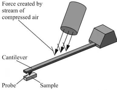
The AFM consists of several systems: a sample positioning system, a mechanical sensor (cantilever) with a scanning tip and a measurement system. All of the systems within the AFM are interdependent of each other. The mechanical part of the AFM sensor consists of an approximately 10-micrometer long tip, which is attached to a long thin cantilever. The surface properties in contact mode AFM are revealed by observing the cantilever deflections caused by the tip – sample interaction. The deflection of the cantilever usually is measured using optical methods. A laser beam is projected on the upper surface of the cantilever close to the tip. The reflected beam is directed via a mirror into an optical sensor [18-20].
Figure 1. Schematics of AFM mechanical sensor system
2.1. Dynamic model
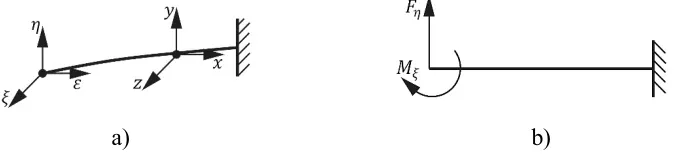
Dynamic model of the system is shown in Figure 2.
Figure 2. Dynamic model of the AFM mechanical sensor system.
The cantilever, which can be assumed as a rod with rectangular cross-section, is approximated by two elastic elements with a concentrated mass at the ends. It is assumed that each element has a mass, and a moment of inertia, which are used to evaluate the deflection and rotation angle of the rod's end. In the lumped mass model, the mass of each element is transferred to the end point of the elastic element as shown in fig 2. It is assumed that the end point is shifted approximately 25,5% of the element's mass [21]. Therefore, the moment of the rod's inertia around its attachment point is evaluated. Supposing that the cantilever is made from silicon nitride Si3N4; the properties of this material correspond to the Kelvin-Voigt material model. The dynamic characteristics of the probe are approximately estimated as elastic elements with damping. The main system coordinates are η1, γ1, η2, γ2, and they describe linear and rotational displacements of cantilever points of interest. The initial clamping force of the cantilever is approximated by a constant force F2, which acts in the negative coordinate η2 direction. The model also includes a nonlinear force F1, introduced by the airflow. This force depends on the gap size between the air supply tube and the cantilever surface.
0 1
1 f
F
,
(1)The roughness of the sample surface, which kinematically excites system oscillations [22], is described by coordinate δ. The probe is approximated by an elastic element with the coefficient of stiffness k, and damping with the coefficient of damping h. The elasticity of the cantilever is evaluated by using the cross-section parameter E Isk, where E – Young’s modulus, Isk = w t3/12 – moment of inertia of the cross-section of the beam with respect to the horizontal axis, where w – width of cantilever and t –thickness of cantilever. It is considered that linear probe movements are described by coordinate η2. The mathematical model is created using Lagrange equations of the second type in the matrix form
A
q
B
q
C
q
Q
,
(2)where [A] – matrix of inertia forces; [B] – matrix of damping coefficients; [C] – matrix of
stiffness coefficients;
T
q
}
1,
1,
2,
2{
– vector of generalized coordinates; {Q} – vector ofgeneralized forces.
Kinetic energy of the system:
.
2
1
22 2 2 2 2 2 1 1 2 1
1
I
m
I
m
T
(3)The matrix of inertia is given as
2 2 1 1
0 0 0
0 0
0
0 0 0
0 0 0
I m I m
A
.
(4)Potential energy is found using methodology [20] as shown in figure 3a.
a)
b)
Figure 3. a) Local coordinates of the beam for potential energy evaluation; b) local generalized coordinates of the beam.
It is considered that in its natural state, the rod is rectilinear and bending occurs only in one plane, as illustrated in Figure 3b. In this case, potential energy of the beam is:
L
sk
ds
EI
sF
M
0
2
2
1
,
(5)In this case, the local generalized coordinates of the beam are force Fη and bending moment Mξ. By differentiating the potential energy of the beam with respect to the generalized coordinates Fη and Mξ the matrix of flexibility is obtained:
sk sk sk skEI
L
EI
L
EI
L
EI
L
2
2
3
2 2 3
.
(6)Matrix of stiffness:
L
EI
L
EI
L
EI
L
EI
C
sk sk sk skstiff
6
4
6
12
2 2 3 1
.
(7)Because the cantilever of the AFM system is modelled by two elements, the ith element of the matrix of stiffness is:
i sk i sk i sk i sk stiffL
EI
L
EI
L
EI
L
EI
C
i
6
4
6
12
2
2 3
.
(8)In our case, the cross-section of the beams and the Young’s modulus are equal for both elements. The potential energy of the cantilever is given by:
2 1 2 1 i iCan
,
(9)where πi – potential energy of ith beam of cantilever,
1 1 1 11 2 ; 1
1
Cstiff
,
(10)
1 2 1 2 1 2 1 22 2 ; 2
1
Cstiff
,
(11)Total potential energy of the mechanical sensor of AFM:
3
Where Π3 – potential energy of the AFM sensor stiffness
22 3
2
1
k
(13)The coefficient of stiffness k is piece-wise linear. To evaluate processes that occur during calculations: when the spring is compressed, k = k0; when the spring is uncompressed, k = 0. This way two different states of the system are obtained. The coefficient of stiffness of the one system states is obtained by differentiating potential energy Π with respect to generalized coordinates η1, γ1, η2, γ2.
2 2 2 2 2 2 2 2 2 3 2 2 2 3 2 2 2 2 2 1 2 2 2 1 2 2 3 2 2 2 2 1 3 2 3 18
12
8
12
12
24
12
24
8
12
8
8
12
12
12
24
12
12
24
24
L
EI
L
EI
L
EI
L
EI
L
EI
L
EI
k
L
EI
L
EI
L
EI
L
EI
L
EI
L
EI
L
EI
L
EI
L
EI
L
EI
L
EI
L
EI
L
EI
L
EI
C
sk sk sk sk sk sk sk sk sk sk sk sk sk sk sk sk sk sk sk sk
(14)The matrix of stiffness for other states of the system differs from the previous state only that here k = 0. It is considered that damping matrix is
B
C (15)where α – constant, and in our case, its value is 0.0009.
The α value is determined from the results of experimental research and has no definite physical meaning. Such a method of proportional damping of the stiffness is often used in systems with an experimentally defined general coefficient of stiffness.
Finally, the vector of generalized forces is:
0 0 2 1
h kF F
Q (16)
.
0
;
24
24
;
0
;
2 44 2 43 2 42 1 41 2 44 2 43 1 42 1 41 2 2 2 2 34 2 2 3 2 1 32 1 31 2 34 2 2 3 2 1 32 1 31 2 2 2 24 2 23 2 22 1 21 2 24 2 23 1 22 1 21 1 1 1 2 14 2 13 1 12 1 11 2 14 2 13 1 12 1 11 1 1
C
C
C
C
B
B
B
B
I
h
k
F
C
k
L
EI
C
C
B
h
L
EI
B
B
m
C
C
C
C
B
B
B
B
I
F
C
C
C
C
B
B
B
B
m
sk sk
(17)where h = α k.
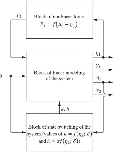
In the other state of the system, the difference between equations is in the values of k = 0 and h = 0. The given equations are solved with respect to the second derivatives of generalized coordinates. From each equation, the corresponding structural diagram and the Matlab/Simulink model is formed. All of these diagrams, representing the corresponding equations, are joined into the general structural diagram. Nonlinear elements in the equations are excluded into different blocks. The simplified structural schematic is presented in Figure 4.
Figure 4. Schematic Simulink diagram of mathematical model: δ – coordinate of kinematic excitation, η1, γ1, η2, γ2 – output coordinates.
The parameters of the aerodynamic force were determined using our previous research results from the theoretical 3D model of the microscope cantilever [17]. This model provided the dependencies among the air gap, the pressure of compressed air and the resulting force on the cantilever. The displacement of the cantilever at coordinate
η
2(Figure 2) was calculated by:η
2= -0.0007 ·
0
1
3+ 0.0033 ·
0
1
2+ 0.0063 ·
0
1
+ 0.0049
(18)3. Experimental technique
Experiments were performed in the Laboratory of Center for physical sciences and technology, using home-made AFM. An AFM cantilever was attached to a displacement measurement system URS143 using a specially designed holder with an installed air duct in order to supply compressed air to the cantilever’s work area (Figure 5). The holder with an installed 0.4 mm diameter air duct inside was designed in accordance with two basic requirements: the duct must not interfere with the optical displacement measurement system; the air stream which flows from the air duct should create a maximum possible aerodynamic force on the upper surface of the cantilever. Additionally, an evaluation of the right size of micro tube was performed by theoretical research on the results of additional air flow simulation performed using FEM [12].
For the precise supply of clean compressed air, a special mechatronic system was designed (Figure 5). The pressure of compressed air in the system is controlled by changing the efficiency of the micro compressor according to the desired pressure and output pressure measured using the pressure sensor MPXV5050GP (Freescale Semiconductor, Austin, TX, USA).
For the control of the whole test rig, measurement system adjustment, calibration and result processing, the LabView software package was used. The control program allows to simultaneously adjust the pressure of compressed air and measure displacement of the cantilever with respect to time. Measurements data was recorded using National instruments data acquisition equipment. During the experiment, compressed air was applied on the upper side of the cantilever. In order to evaluate the effect of sample surface, a piece of glass was placed at few micrometers under the probe. Air pressure was increased from 0 kPa to 20 kPa by step size 1 kPa, and the response of the cantilever was measured.
a) b)
Figure 5. Experimental equipment: a) air supply system, b) holder
In order to ensure repeatability of further researches and to create a possibility to scan the same structures with different speeds, there were special samples manufactured with periodic structures as shown in Figure 6. The period of structures was changed in a range from 1 μm to 9 μm.
a) b) c)
Figure 6. Photolithography mask: a) common view, b) view of one square from a) part, c) zoomed view of four squares
Samples were fabricated using photolithography. First, a chromium layer of 50 nm thickness was developed on a borosilicate glass wafer (700 μm thickness). Using a photolithography mask (Figure 6), the chromium layer was covered by photoresist. Then the layer of chromium was etched for 3 min. Finally, the photoresist was removed. The structure quality was measured using a 3D Laser Scanning Confocal Microscope VK-X260K from KEYENCE America (Itasca, IL, USA) with a vertical resolution of 0.5 nm.
4. Results and discussion
4.1. Experimental results
4.1.1. Measurements by laser scanning microscope
Laser Scanning Confocal Microscope (LSCM) was used for the measurement of fabricated structures. A fabricated structure is uneven and has sharp edges (Figure 7). It is not easy to measure such structures by AFM, therefore, we expected that the AFM picture will show ‘loss of contact’ between the tip and the sample’s surface, or some inaccuracy. Moreover, an(?) ideal surface, when it is used as input in the model, allows to get a response from the AFM model in a natural way. Sometimes, if the roughness of the surface is not known, it is hard to decide about imaging artifacts.
b)
Figure 7. Fabricated structures, measured by LSCM: a) scanned structure from Figure 6, period 2 μm; b) scanned structure from Figure 6, period 9 μm.
Therefore, the results observed by LSCM are useful, since knowing real structure made the AFM experiment more clear and reliable. Data from this measurement is used as control patterns for further research.
4.1.2. Measurements by atomic force microscope
Experiments with home-made AFM were performed in the same way as using LSCM. The whole surface was scanned at 112.5 μm/s speed in contact mode, and one line was chosen for model input (Figure 8). Dependency between the surface point coordinate and the structure profile height was converted to dependency between time and profile height as shown in Figure 8 b. This conversion is needed in order to use this dependency as an input for the model, and to simulate cases when the same sample is scanned at various speeds using different cantilevers. Comparing the AFM and LSCM results, it was observed that the results of structure topography are similar: the average surface roughness is 50 nm; the distance between the peaks of profile is 3 μm.
a) b)
Figure 8. a) Error signal map of scanned surface; b) Horizontal scanning data from a), white line. Scanning speed 112.5 μm/s.
4.1.3. Effect of applied pressure to vertical displacement of the cantilever
explanation of our suggested modification and research on the additional force was presented in [12]. It is important to choose appropriate gas for the pressure system, therefore, in our earlier research there were calculated dependencies of distance versus displacement using carbon monoxide, nitrogen, air, and argon [17]. It was found that the highest displacement could be observed using carbon monoxide. Using air, nitrogen, and argon, the displacement is quite similar. However, the easiest way to apply pressure to the cantilever is to use compressed air.
Experimental research with an applied stabilizing air stream was performed according to the following methodology: pressure of applied compressed air stream was changed in the range 0…20 kPa with pitch of 1 kPa, and displacement (change in coordinate η2, Figure 2) of the cantilever (Table 1, Case 1: soft rectangular cantilever) was measured. The dependencies between set pressure, real pressure and cantilever displacement are shown in Figure 9. Set pressure is different from real pressure due to the properties of air supply and the control system of stream pressure regulator. Air pressure in the system and cantilever displacement were measured continuously during the whole experiment. When the pressure of compressed air was increasing from 0 to 12 kPa, the displacement of the cantilever increased linearly from 0 to 4 μm. When the pressure of compressed air was increased more than 12 kPa, the displacement of the cantilever decreases significantly. In this case, air flow creates a lifting force between the cantilever’s lower surface and the sample surface, which compensates for the aerodynamic force (F1, Figure 2), developed on the cantilever’s upper surface.
Figure 9. Cantilever’s vertical displacement at different applied pressures.
The performed experimental test of aerodynamic force implementation into the AFM cantilever control reveals a range of useful air pressure for our modified AFM measurement sensor as 1…12 kPa.
The experimental setup gives stable and permanent values of air stream, therefore to repeat this experiment, it is needed to adjust the pneumatic duct to the particular design of AFM. Also, it is necessary to state that the calibration of the aerodynamic system is required after each change of components of AFM sensors.
4.2. Analytical results
4.2.1. AFM contact mode simulation
Simulations were performed using the AFM horizontal contact mode scanning result (Figure 8 b) as a model input. The AFM dynamic system was simulated in two cases: the initial and aerodynamically loaded models. The applied aerodynamic load represents the air flow from the microscopic tube. Model parameters, used in the simulation, are provided in Table 1. In order to achieve the desired stiffness of the cantilever, an additional force from the air stream, treated as supplemental stiffness of the cantilever in the dynamical model; the pressure in the air supply system is set to 60 Pa. This value is taken from experimental results (Figure 9). This value of supply pressure is necessary due to the compensation of aerodynamically lost air, initially supplied by a 4 mm diameter tube, through a 0.6 mm connector to a 0.4 mm air duct in a holder. This is necessary to explain that these two different values of pressure apply to a different part of the pneumatic system. The value of 60 Pa relates to the outlet air stream from the thin duct in close position to the AFM cantilever. The high value of pressure is applied to the input of the special air duct, and its effective value can be measured by a real gauge.
The relation between these two pressures was detected indirectly. First, the FEM model of the air duct system, and the aerodynamic chamber between the duct outlet and the corresponding cantilever surface, modelled in the steady-state task, and material on this research is provided in [12]. The experimental definition of outlet pressure from the duct is practically impossible, therefore an indirect method was used. The pneumatic system was installed in the real AFM sensor, and deflections of the sensor were measured only with an aerodynamic force load. Having real stiffness of a sensor cantilever, the value of aerodynamic force was detected.
Taking into account both of these circumstances, in the model the lowest value of air stream was supplied based on the experimental aerodynamic force of it. In the experimental research, the highest value of air pressure was used only as a possible control value.
Table 1. Main parameters of modelled cantilevers
Parameter Case 1: soft rectangular
cantilever
Case 2: stiff rectangular cantilever
Constant, α 0.0009 0.0009
Length, L 450 μm 117 μm
Mass, m1 9.5310-11 kg 5.3110-11 kg
Mass, m2 4,7710-11 kg 2.6510-11 kg
Resonant Frequency, f 13 kHz 320 kHz
Size of the initial gap, Δ0
0.4 mm 0.4 mm
Spring Constant, k 0.2 N/m 40 N/m
Thickness, t 2 μm 3.5 μm
Width, w 50 μm 33 μm
Young’s modulus, E 310 GPa 310 GPa
To determine the effect of an additional stiffness, the same model was solved with and without the additional nonlinear stiffness element added. A comparison of simulation results allows to identify the AFM system's change of its dynamic characteristics, due to the additional nonlinear controllable stiffness element.
4.2.1. Results of AFM contact mode simulation
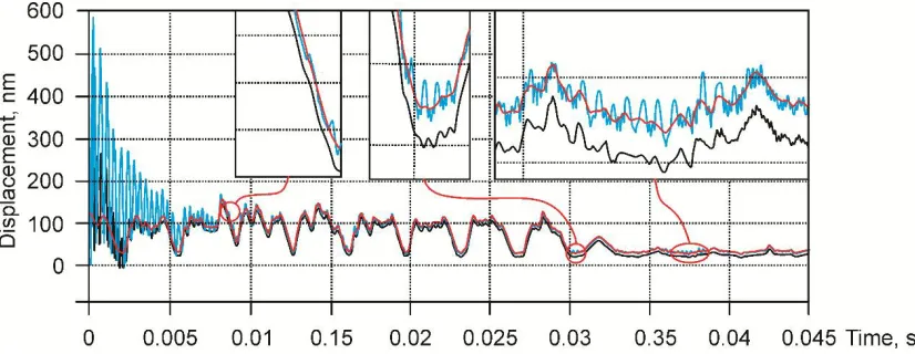
Figure 10. The displacement of the soft cantilever's (case 1 in the Table 1) response to excitation, defined using experimental data from Figure 8 b as an input signal. Scanning speed 112 μm/s; red- excitation signal; blue - response of non-modified AFM sensor; black - response of modified sensor.
The next simulation done at a speed, ten times higher than the previous one, with the same pressure applied (Figure 11). The model output was observed for the modified AFM sensor, which was negatively offset if compared to the excitation and output for the non-modified AFM sensor. Also, as seen in the insets of the Figure 11, the output for the modified AFM sensor contains less small-scale noise, which is observed in the output for the non-modified AFM sensor. This small-scale improvement is explained as yet another result of the applied pressure.
Figure 11. The displacement of the soft cantilever's (case 1 in the Table 1) response to excitation, defined using experimental data from Figure 8 b as an input signal. Scanning speed 1120 μm/s, applied pressure 60 Pa; red - excitation signal; blue - response of non-modified AFM sensor; black - response of modified sensor.
Figure 12. The displacement of the soft cantilever's (case 1 in the Table 1) response to excitation, obtained using experimental data from Figure 8 b as an input signal. Scanning speed 1120 μm/s, applied pressure 40.0 Pa. red- excitation signal; blue - response of non-modified AFM sensor; black - response of modified sensor.
Low pressure influence on the sensor signal revealed itself only on landscape extremities; nevertheless it can be useful for soft sample scanning.
Figure 13. The displacement of the soft cantilever's (case 1 in the Table 1) response to excitation, obtained using experimental data from Figure 8 b as an input signal. Scanning speed 1120 μm/s, applied pressure 20.0 Pa. Red - excitation signal; blue - response of non-modified AFM sensor; black - response of modified sensor.
Figure 14. The displacement of the stiff cantilever's (case 2 in the Table 1) response to excitation, obtained using experimental data from Figure 8 b as an input signal. Scanning speed 112 μm/s, applied pressure 60 Pa; 1- excitation signal; 2- response of non-modified AFM sensor; 3- response of modified sensor.
We observed contact loss only applying at much higher speed: 11.2 mm/s (Figure 15 a), and 11.2 m/s (Figure 15 b). At 11.2 mm/s the speed contact loss is seen from 0 to 1.04 s (Figure 15 a). However, from 0 to 0.8 s, there is noise from the model, which under some conditions can be observed at the start of simulation. The contact loss in practice usually occurs at the peaks and valleys at high speeds. Therefore, we compare the responses of original and modified sensors obtained at the highest peak (0.826 s). It was found that displacement using a non-modified sensor is 180 nm, and displacement obtained with a modified sensor is 151 nm, while the value of the excitation signal at this time point is 148 nm. Therefore, the difference between the response and excitation signals is 32 nm for a non-modified sensor, and only 3 nm when the modified sensor is used. Thus, our method at the speed of 11 mm/s gives an accuracy of 11 times more, compared to the usual AFM.
A much better result at 11.2 m/s scanning speed was obtained (Figure 15 b). It is seen from Figure 15 b that applying a high speed to the cantilever’s tip gives very high displacement, two times higher than the input signal. However, the sensor with applied pressure shows the response close to the input signal. Comparing results at 1.4 s, there was observed displacement 240 nm using a non-modified sensor, and 149 nm using a modified sensor, while the value of the excitation signal at this point is 148 nm. Therefore, the difference between excitation and response for the non-modified sensor is 92 nm, while for the modified sensor it is only 1 nm. Thus, the vertical accuracy can be estimated as 92 times more than the usual AFM.
Figure 15. The displacement of the stiff cantilever's (case 2 in the Table 1) response to excitation, obtained using experimental data from Figure 8 b as an input signal. a) scanning speed 11.2 mm/s, b) scanning speed 11.2 m/s. Applied pressure 60 Pa; 1- excitation signal; 2- response of non-modified AFM sensor; 3- response of modified sensor.
The figure 15 b) shows the outputs of the model for the scanning speed, which is 105 times higher than the standard scanning speed. Here kinematic excitation of the unmodified AFM sensor approaches its resonant frequency (which is 320 kHz), and the oscillating character of the sensor response is seen. At the same time, the output of the modified AFM sensor remains intact, which we attribute to the effect of applied air stream.
5. Conclusions
Implementation of air stream as a nonlinear spring in the AFM sensor mechanical part demonstrated promising results: 11 times better vertical accuracy if compared with the unmodified AFM sensor working at 11.2 mm/s (equivalent to 24 lines/s at 50 μm field of view) scanning speed, while the standard scanning speed of the particular AFM system is 112 μ/s (2.4 lines/s at 50 μm field of view). Our model shows that by using the modified AFM sensor, there is a potential to improve the accuracy of the vertical axis as much as 92 times if a stiff cantilever (spring constant of 40 N/m) is used. Efficiency of applying the non-linear additional stiffness depends on the stiffness and geometric parameters of the sensor cantilevers. The softer cantilever (spring constant of 0.2 N/m) in the case of the unmodified AFM sensor exhibits undesired oscillatory behavior already at 1.12 mm/s scanning speed, which provides an excitation close to the resonance frequency of the cantilever (which is 13 kHz). Our model shows that the signal can be improved by applying 20 Pa pressure. The same unmodified AFM sensor, if coupled with the stiff cantilever, will start to exhibit similar oscillatory behavior at 11.2 mm/s, for the same reason of excitation approaching the resonant frequency (320 kHz in this case). This undesired behavior can be eliminated by applying 60 Pa pressure. Modification of the sensor, by applying the air stream, creates the potential for an effective increase of the scanning speed of at least 10 times more, if a soft cantilever is used. Also, in the case of a stiff cantilever, the potential of the scanning speed improvement is at least 100 times. We claim our method to be efficient when the kinematic excitation, caused by the increased scanning speed, will excite oscillating behavior of the sensor.
Our model also shows that there is a potential of an effective increase of the scanning speed up to 11.2 m/s, however this is rarely practically possible in the physical AFM systems.
We also see some limitations and drawbacks of the proposed method. First of all, the effect of the non-linear force applied to the cantilever is limited when lower values (more than 100 nm) are to be imaged. Second, the minimum pressure from the air stream is limited to 20 Pa in the case of the soft cantilever to be effective. In the case of the stiff cantilever, this bottom limit is higher. Also, the maximum useful pressure is limited to 60 Pa in the case of the stiff cantilever, because higher pressure will decrease the accuracy of the sensor. Correspondingly, for soft cantilevers this upper limit will be lower.
The proposed dynamic model of the AFM sensor reproduces the experimental results well. So, it can be used to predict scanning modes and to provide a scan parameter estimation for other kinds of modified AFM sensors.
Acknowledgments: This work is a part of Andrius Dzedzickis PhD project “Modeling of mechanical structure of Atomic force microscope sensor and research of its dynamic characteristics”.
Author Contributions: All authors equally contributed to this article.
References
1. Janickis, V.; Petrašauskienė, N.; Žalenkienė, S.; Morkvėnaitė-Vilkončienė, I.; Ramanavičius, A. Morphology of cdse-based coatings formed on polyamide substrate. Journal of Nanoscience and Nanotechnology 2018, 18, 604-613. http://dx.doi.org/10.1166/jnn.2018.13927.
2. Morkvenaite-Vilkonciene, I.; Ramanaviciene, A.; Genys, P.; Ramanavicius, A. Evaluation of enzymatic kinetics of gox-based electrodes by scanning electrochemical microscopy at redox competition mode. Electroanalysis 2017. http://dx.doi.org/10.1002/elan.201700022.
3. Morkvenaite-Vilkonciene, I.; Ramanavicius, A.; Ramanaviciene, A. Atomic force microscopy as a tool for the investigation of living cells. Medicina 2013, 49, 155-164.
4. Ulčinas, A.; Vaitekonis, Š. Rotational scanning atomic force microscopy. Nanotechnology 2017, 28, 10LT02. http://dx.doi.org/10.1088/1361-6528/aa5af7.
5. Adams, J.D.; Nievergelt, A.; Erickson, B.W.; Yang, C.; Dukic, M.; Fantner, G.E. High-speed imaging upgrade for a standard sample scanning atomic force microscope using small cantilevers. Rev. Sci. Instrum. 2014, 85, 093702. http://dx.doi.org/10.1063/1.4895460.
6. Akrami, S.M.; Miyata, K.; Asakawa, H.; Fukuma, T. Note: High-speed z tip scanner with screw cantilever holding mechanism for atomic-resolution atomic force microscopy in liquid. Rev. Sci. Instrum. 2014, 85, 126106. http://dx.doi.org/10.1063/1.4904029.
7. Leitner, M.; Fantner, G.E.; Fantner, E.J.; Ivanova, K.; Ivanov, T.; Rangelow, I.; Ebner, A.; Rangl, M.; Tang, J.; Hinterdorfer, P. Increased imaging speed and force sensitivity for bio-applications with small cantilevers using a conventional afm setup. Micron 2012, 43, 1399-1407. http://dx.doi.org/10.1016/j.micron.2012.05.007.
8. Hosaka, S.; Etoh, K.; Kikukawa, A.; Koyanagi, H.; Itoh, K. 6.6 mhz silicon afm cantilever for high-speed readout in afm-based recording. Microelectron. Eng. 1999, 46, 109-112. http://dx.doi.org/10.1016/S0167-9317(99)00027-1.
9. Michels, T.; Guliyev, E.; Klukowski, M.; W. Rangelow, I. Micromachined self-actuated piezoresistive cantilever for high speed spm. Microelectron. Eng. 2012, 97, 265-268. http://dx.doi.org/10.1016/j.mee.2012.03.029. 10. Balantekin, M. High-speed dynamic atomic force microscopy by using a q-controlled cantilever eigenmode as an actuator. Ultramicroscopy 2015, 149, 45-50. http://dx.doi.org/10.1016/j.ultramic.2014.11.016. 11. Bučinskas, V.; Dzedzickis, A.; Šešok, N.; Šutinys, E.; Iljin, I. Research of modified mechanical sensor of atomic force microscope. In Dynamical systems: Theoretical and experimental analysis: Łódź, poland, december 7-10, 2015, Awrejcewicz, J., Ed. Springer International Publishing: Cham, 2016; pp 39-48.
12. Dzedzickis, A., Bučinskas, Vytautas, Šešok, Nikolaj, Iljin, Igor. Modelling of mechanical structure of atomic force microscope. Solid State Phenomena 2016, 251, 77-82. http://dx.doi.org/10.4028/www.scientific.net/SSP.251.77.
13. Theisen, L.R.S.; Niemann, H.H.; Galeazzi, R.; Santos, I.F. Enhancing damping of gas bearings using linear parameter-varying control. Journal of Sound and Vibration 2017, 395, 48-64. http://dx.doi.org/10.1016/j.jsv.2017.02.021.
14. Shen, I.Y. Recent vibration issues in computer hard disk drives. J. Magn. Magn. Mater. 2000, 209, 6-9. http://dx.doi.org/10.1016/S0304-8853(99)00633-2.
15. Müller, C.; Greco, S.; Kirsch, B.; Aurich, J.C. A finite element analysis of air bearings applied in compact air bearing spindles. Procedia CIRP 2017, 58, 607-612. http://dx.doi.org/10.1016/j.procir.2017.03.337.
16. Kubotera, H.; Tsuda, N.; Tatewaki, M.; Maruyama, T. Aerodynamic vibration mechanism of hdd arms predicted by unsteady numerical simulations. IEEE transactions on magnetics 2002, 38, 2201-2203. http://dx.doi.org/10.1109/TMAG.2002.801866.
17. Bučinskas, V.; Dzedzickis, A.; Šutinys, E.; Lenkutis, T. Implementation of different gas influence for operation of modified atomic force microscope sensor. Solid State Phenomena 2017, 260. http://dx.doi.org/10.4028/www.scientific.net/SSP.260.99.
18. Lu, H.; Fang, Y.; Ren, X.; Zhang, X. Improved direct inverse tracking control of a piezoelectric tube scanner for high-speed afm imaging. Mechatronics 2015, 31, 189-195. http://dx.doi.org/10.1016/j.mechatronics.2015.08.006.
20. Martin, M.J.; Fathy, H.K.; Houston, B.H. Dynamic simulation of atomic force microscope cantilevers oscillating in liquid. J. Appl. Phys. 2008, 104, 044316. http://dx.doi.org/10.1063/1.2970154.
21. Augustaitis, V.; Gičan, V.; Šešok, N.; Iljin, I. Computer-aided generation of equations and structural diagrams for simulation of linear stationary mechanical dynamic systems. Mechanics 2011, 17, 255-263. http://dx.doi.org/10.5755/j01.mech.17.3.500.
22. Zhang, Y.; Zhao, Y.-p. Nonlinear dynamics of atomic force microscopy with intermittent contact. Chaos, Solitons & Fractals 2007, 34, 1021-1024. http://dx.doi.org/10.1016/j.chaos.2006.03.125.