Summation polynomial algorithms for elliptic curves in characteristic two
Steven D. Galbraith and Shishay W. Gebregiyorgis
Mathematics Department, University of Auckland,
New Zealand.
[email protected],[email protected]
Abstract. The paper is about the discrete logarithm problem for elliptic curves over characteristic 2 finite fields
F2nof prime degreen. We consider practical issues about index calculus attacks using summation polynomials in
this setting. The contributions of the paper include: a choice of variables for binary Edwards curves (invariant under the action of a relatively large group) to lower the degree of the summation polynomials; a choice of factor base that “breaks symmetry” and increases the probability of finding a relation; an experimental investigation of the use of SAT solvers rather than Gr¨obner basis methods for solving multivariate polynomial equations overF2.
We show that our choice of variables gives a significant improvement to previous work in this case. The symmetry-breaking factor base and use of SAT solvers seem to give some benefits in practice, but our experimental results are not conclusive. Our work indicates that Pollard rho is still much faster than index calculus algorithms for the ECDLP (and even for variants such as the oracle-assisted static Diffie-Hellman problem of Granger and Joux-Vitse) over prime extension fieldsF2nof reasonable size.
Keywords:ECDLP, summation polynomials, index calculus.
1 Introduction
LetE be an elliptic curve over a finite field F2n wheren is prime. The elliptic curve discrete logarithm problem (ECDLP) is: Given P, Q ∈ E(F2n) to compute an integer a, if it exists, such that Q = aP. As is standard, we restrict attention to pointsP of prime orderr. The Diffie-Hellman problem (CDH) is: Given P ∈ E(F2n) and points P1 = aP and P2 = bP, for some integers a and b, to computeabP. These two computational problems are fundamental to elliptic curve cryptography. There is a wide variety of “interactive” Diffie-Hellman assumptions, meaning that the attacker/solver is given access to an oracle that will perform various computations for them. These problems also arise in some cryptographic settings, and it is interesting to study them (for scenarios where they arise in practice for static-CDH see Brown and Gallant [3]). These problems are surveyed by Koblitz and Menezes [23] and we recall some of them now.
– The “Delayed Target One-More Discrete Logarithm Problem” in the sense of Joux-Naccache-Thom´e is the following. The solver is supplied with a discrete logarithm oracle and must find the discrete logarithm of a random group elementY that is given to the solver only after all the queries to the oracle have been made.
– The “oracle-assisted static Hellman problem” (also called the “delayed target One-More Diffie-Hellman problem”) is the following. The solver is given(P, X = aP) and a static (also called “one-sided”) Diffie-Hellman oracle (i.e.,O(Y) =aY), and must solve the DHP with input(P, X, Y), where
Y is a random group element that is given to the solver only after all the queries toOhave been made. In other words, the solver must computeZ =aY.
– The “static One-More Diffie-Hellman Problem” is as follows. The solver is again given(P, X =aP)
and access to an oracleO(Y) = aY, and also a challenge oracle that produces random group elements
Early papers on attacking these sorts of interactive assumptions (e.g., [20]) used index calculus algo-rithms for finite fields. Granger [18] and Joux-Vitse [22] were the first to consider the case of elliptic curve groupsE(Fqn) (both papers mainly focus on the case whereqis a large prime, and briefly mention small characteristic but not prime degree extension fieldsF2n).
One approach to solving the ECDLP (or these interactive assumptions) is to use Semaev’s summation polynomials [27] and index calculus ideas of Gaudry, Diem, and others [5–8, 11–13, 16, 21, 22, 25]. The main idea is to specify a factor base and then to try and “decompose” random pointsR =uP +wQas a sumP1+· · ·+Pmof points in the factor base. Semaev’s summation polynomials allow to express the sum
P1+· · ·+Pm −R = ∞, where∞is the identity element, as a polynomial equation overF2n, and then Weil descent reduces this problem to a system of polynomial equations overF2
There is a growing literature on these algorithms. Much of the previous research has been focussed on elliptic curves overFqnwhereqis prime or a prime power, andnis small.
Our Work This paper is about the caseF2n where nis prime. Other work (for example [6–8, 25]) has focused on asymptotic results and theoretical considerations. Instead, we focus on very practical issues and ask about what can actually be computed in practice today. In other words, we follow the same approach as Huang, Petit, Shinohara and Takagi [19] and Shantz and Teske [26].
We assume throughout that the ECDLP instance cannot be efficiently solved using the Gaudry-Hess-Smart approach [15] or its extensions, and that the point decomposition step of the algorithm is the bottle-neck (so we ignore the cost of the linear algebra). This will be the case in our examples.
The goal of our paper is to report on our experiments with three ideas:
(1) We describe a choice of variables for binary Edwards curves that is invariant under the action of a relatively large group (generated by the action of the symmetric group and addition by a point of order 4). This allows the summation polynomials to be re-written with lower degree, which in turn speeds up the computation of relations.
(2)We consider a factor base that “breaks symmetry” and hence significantly increases the probability that relations exist. It may seem counterintuitive that one can use symmetric variables to reduce the degree and also a non-symmetric factor base, but if one designs the factor base correctly then this is seen to be possible. The basic idea is as follows. The traditional approach has relationsR = P1 +· · ·+Pm wherePi ∈
F ={P ∈E(F2n) : x(P) ∈V}whereV ⊆F2n is someF2-vector subspace of dimensionl. Instead, we demandPi ∈ Fi over1 ≤ i ≤ m form different factor basesFi = {P ∈ E(F2n) : x(P) ∈ V +vi} wherevi ∈ F2n are elements of a certain form so that the setsV +vi are all distinct. (Diem [8] has also used different factor basesFi, but in a different way.) The probability of finding a relation is increased by a factor approximatelym!, but we needmtimes as many relations, so the total speedup is approximately by a factor of(m−1)!.
(3)We experiment with SAT solvers rather than Gr¨obner basis methods for solving the polynomial systems. This is possible since we obtain a system of multivariate polynomial equations overF2, rather than over larger fields. (SAT solvers have been considered in cryptanalysis before, e.g. [4, 24].)
Our conclusions are: The suggested coordinates for binary Edwards curves give a significant improve-ment over previous work on elliptic curves in characteristic 2. The use of SAT solvers may potentially enable larger factor bases to be considered (however, it seems an “early abort” strategy should be taken, as we will explain). Symmetry breaking seems to give a moderate benefit whennis large compared withlm.
earlier) in characteristic 2 elliptic curves than to use Pollard rho. Hence, summation polynomial algorithms do not seem to be a useful tool for attacking current ECDLP challenge curves for curves defined overF2n wherenis prime.
The paper is organised as follows. Section 2 recalls previous work. Section 3 recalls binary Edwards curves and introduces our new variables. Section 4 shows how to do the index calculus attack in this setting and discusses the symmetry-breaking idea. Section 5 discusses the use of SAT solvers, while Section 6 reports on our experimental results.
2 Index Calculus Algorithms and Summation Polynomials
We briefly recall the basic ideas of these methods and introduce our notation. LetP ∈E(F2n)have prime orderrand supposeQ=aP. One chooses an appropriate factor baseF ⊆E(F2n), computes random points
R =uP +wQand then tries to writeR =P1+· · ·+Pm forPi ∈ F. Each successful decomposition of the pointRis called a “relation”. Let`= #F. WritingF ={F1, . . . , F`}we can write thej-th relation as
ujP+wjQ=P`i=1zj,iFiand store the relation by storing the values(uj, wj)and the vector(zj,1, . . . , zj,`). When enough relations (more than`) are found then one can apply (sparse) linear algebra to find a kernel vector of the matrixM = (zj,i)and hence obtain a pair of integersuandwsuch thatuP +wQ= 0from which we can solve fora≡ −uw−1 (modr)as long asw6≡0 (modr). The details are standard.
One can use this approach to solve interactive Diffie-Hellman assumptions. We give the details in the case of the oracle-assisted static Diffie-Hellman. Choose a factor baseF ={F1, . . . , F`}then call the oracle for each elementFi to get the points aFi for 1 ≤ i ≤ `. When provided with the challenge pointY one tries to decomposeY =P1+· · ·+Pmfor pointsPi ∈ F. If such a relation is found then we can compute the required pointaY asaP1+· · ·+aPm. (If we fail to find a relation then we can randomise by taking
Y +uP and recalling thatuX =uaP.)
One sees that all applications require decomposing random points over the factor base. This is the dif-ficult part of the algorithm and is the main focus of our paper. Note however that the ECDLP application requires a very large number of relations and hence a very large number of point decompositions, whereas the oracle-assisted static-DH application only requires a single relation.
We will ignore the linear algebra step as, for the parameters considered in the paper, its cost will always be insignificant.
2.1 Summation Polynomials
Let E be an elliptic curve in Weierstrass form over a field K of odd characteristic. The mth summation
polynomial fm(x1, x2, . . . , xm) ∈ K[x1, x2, . . . , xm] for E, defined by Semaev [27], has the following defining property. Let X1, X2, . . . , Xm ∈ K. Then fm(X1, X2, . . . , Xm) = 0 if and only if there exist
Y1, Y2, . . . , Ym ∈ K such that (Xi, Yi) ∈ E(K) for all 1 ≤ i ≤ m and (X1, Y1) + (X2, Y2) +· · ·+
(Xm, Ym) =∞, where∞is the identity element.
Lemma 1. (Semaev [27]) LetE:y2 =x3+a4x+a6be an elliptic curve over a fieldKof characteristic
6
= 2,3and{a4, a6} ∈K. The summation polynomials forEare given as follows.
f2(X1, X2)=X1−X2
f3(X1, X2, X3)=(X1−X2)2X32−2((X1+X2)(X1X2+a4) + 2a6)X3
Form≥4and a constantjsuch that1≤j≤m−3, then
fm(X1, . . . , Xm) =ResultantX(fm−j(X1, . . . , Xm−j−1, X), fj+2(Xm−j, Xm−j+1, . . . , Xm, X)).
For m ≥ 2, the mth summation polynomial fm is an irreducible symmetric polynomial that has degree
2m−2in each of the variables.
Gaudry and Diem noted that, for elliptic curvesE(Fqn)over extension fields, there are choices of factor base for which the problem of finding solutions to summation polynomials can be approached using Weil descent with respect toFqn/Fq. In other words, the problem of solvingfm+1(x1, . . . , xm, x(R))forxi ∈Fq can be reduced to a system of multivariate polynomial equations overFq. The details are standard.
To solve the system of multivariate polynomial equations, the current most effective approach (see [11, 19]) is to perform theF4 orF5 algorithm for the graded reverse lex order, followed by the FGLM algo-rithm [14].
2.2 Degree Reduction Via Symmetries
The summation polynomials have high degree, which makes solving them difficult. Since the summation polynomial is invariant under the action of the symmetric groupSm, Gaudry [16] observed that re-writing the polynomial in terms of invariant variables reduces the degree and speeds up the resolution of the system of equations. As well as lowering the degree of the polynomials, this idea also makes the solution set smaller and hence faster to compute using the FGLM algorithm.
Faug`ere et al [12, 13] have considered action by larger groups (by using points of small order) for elliptic curves overFqn wherenis small (e.g.,n= 4 orn= 5) and the characteristic is6= 2,3. Their work gives further reduction in the cost of solving the system. We sketch (for all the details see [12, 13]) the case of points of order2on twisted Edwards curves.
For a point P = (x, y) on a twisted Edwards curve we have −P = (−x, y) and so it is natural to construct summation polynomials in terms of the y-coordinate (invariant under P 7→ −P). Accordingly Faug`ere et al [12] define their factor base as
F ={P = (x, y)∈Fqn :y∈Fq}.
Further, the addition ofP with the pointT2 = (0,−1)(which has order 2) satisfiesP +T2 = (−x,−y). Note thatP ∈ F if and only ifP+T2 ∈ F. Hence, for each decompositionR =P1+P2+· · ·+Pn, there exist2n−1further decompositions, such as
R= (P1+T2) + (P2+T2) +P3+· · ·+Pn.
It follows that the dihedral coxeter groupDn= (Z/2Z)n−1oSnof order2n−1n!acts on the set of relations
R=P1+· · ·+Pnfor any given pointR(and all these relations correspond to solutions of the summation polynomial). It is therefore natural to try to write the summation polynomialfn+1(y1, y2, . . . , yn, y(R))in terms of new variables that are invariant under the group action. For further details see [12].
2.3 The Case ofF2n wherenis Prime
Following Diem [8] we define the factor base in terms of anF2-vector spaceV ⊂ F2n of dimensionl. A typical choice for the factor base in the case of Weierstrass curves isF ={P ∈E(F2n) :x(P)∈V}, and one wants to decompose random points asR=P1+· · ·+PmforPi∈ F.
As above, the symmetric groupSmof orderm!acts on the set of relationsR =P1+· · ·+Pmfor any given pointR(and all these relations correspond to solutions of the summation polynomial). It is therefore natural to try to write the summation polynomial fm+1(x1, x2, . . . , xm, x(R)) in terms of new variables that are invariant under the group action. In this example, such variables are the elementary symmetric polynomials in thexi. This approach gives polynomials of lower degree.
Huang et al [19] observe that it is hard to combine re-writing the summation polynomial in terms of symmetric variables and also using a factor base defined with respect to an arbitrary vector subspace of
F2n. The point is that ifx1, . . . , xm ∈V then it is not necessarily the case that the value of the symmetric polynomiale2 =x1x2+x1x3+· · ·+xm−1xm(or higher ones) lies inV. Hence, one might think that one cannot use symmetries in this setting.
Section 3 of [19] considers primenand the new idea of “both symmetric and non-symmetric variables”. It is suggested to use a “special subspace”V that behaves relatively well under multiplication:xi, xj ∈ V implies xixj ∈ V0 for a somewhat larger space V0. The experiments in [19], for n prime in the range
17≤n≤53,m= 3, andl∈ {3,4,5,6}, show a significant decrease of the degree of regularity (the highest degree reached) during Gr¨obner basis computations. However, the decrease in the degree of regularity is at the expense of an increased number of variables, which in turn increases the complexity of the Gr¨obner basis computations (which roughly take timeN3Dand requireN2Dmemory, whereN is the number of variables andDis the degree of regularity).
Huang et al [19] exploit the action of Sm on the summation polynomials but do not exploit points of order 2 or 4. One of our contributions is to give coordinates that allow to exploit larger symmetry groups in the case of elliptic curves over binary fields. We are able to solve larger experiments in this case (e.g., taking decompositions intom = 4points, while [19] could only handle m = 3). For more details of our experiments see Section 6.
3 Edwards Elliptic Curves in Characteristic Two
We study binary Edwards curves [1] since the addition by points of order 2 and 4 is nicer than when using the Weierstrass model as was done in [12, 13]. Hence we feel this model of curves is ideally suited for the index calculus application.
Definition 1. Letd1, d2 ∈ F2n be such that d1 6= 0andd2 6= d21 +d1. The binary Edwards curve with coefficientsd1andd2is the elliptic curve given by the affine model
Ed1,d2 : d1(x+y) +d2(x
2+y2) =xy+xy(x+y) +x2y2.
The binary Edwards curve is symmetric in the variablesxandywith the following group law [1]. 1. The identity element is the pointP0 = (0,0).
2. For a pointP = (x, y)∈Ed1,d2, its negation is given by−P = (y, x). We haveP+−P =P0= (0,0).
3. LetP1= (x1, y1), P2 = (x2, y2)∈Ed1,d2, thenP3 = (x3, y3) =P1+P2is given by x3=
d1(x1+x2) +d2(x1+y1)(x2+y2) + (x1+x21)(x2(y1+y2+ 1) +y1y2)
d1+ (x1+x21)(x2+y2)
y3=
d1(y1+y2) +d2(x1+y1)(x2+y2) + (y1+y21)(y2(x1+x2+ 1) +x1x2)
d1+ (y1+y12)(x2+y2)
4. The pointT2 = (1,1)∈Ed1,d2 is invariant under negation so it has order2. For any pointP = (x, y)∈ Ed1,d2 we haveP+T2 = (x+ 1, y+ 1).
Ifd1 6= 0and TrF2n/F2(d2) = 1, i.e., there is no elementu∈F2nsuch thatusatisfiesu
2+u+d 2= 0, then the addition law on the binary Edwards curve is complete [1]. That is, the denominators in the addition lawd1+ (y1+y21)(x2+y2)andd1+ (x1+x12)(x2+y2)never vanish.
For summation polynomials with these curves, the best choice of variable ist=x+y. This is the natural choice, consistent with previous work [16, 12], as this function is invariant under the action of[−1] : P 7→ −P. The coordinatetwas used in [1] for differential addition, but it was calledω.
The function t : Ed1,d2 → P
1 has degree4. Given a value t ∈
F2n there are generically four points
P = (x, y)∈E(F2)having the same value fort(P), namely(x, y),(y, x),(x+ 1, y+ 1),(y+ 1, x+ 1). When we come to define the factor base, we will choose a vector subspaceV ofF2n/F2of dimensionl and will define the factor base to be the set of points corresponding tot(P) =x(P) +y(P)∈V.
Theorem 1. LetEd1,d2 be a binary Edwards curve overF2n and define the functiont(P) =x(P) +y(P).
Let themthsummation polynomials for binary Edwards curves be defined as follows:
f2(t1, t2)=t1−t2
f3(t1, t2, t3)=(d2t21t22+d1(t21t2+t1t22+t1t2+d1))t23+d1(t21t22+t21t2+t1t22+t1t2)t3
+d21(t21+t22)
fm(t1, . . . , tm)=Resultantt(fm−k(t1, t2, . . . , tm−k−1, t), fk+2(tm−k, tm−k+1, . . . , tm, t)), form≥4and1≤k≤m−3.
For any pointsP1, . . . , Pm ∈Ed1,d2(F2)such thatP1+· · ·+Pm =P0, thenfm(t(P1), . . . , t(Pm)) = 0.
Conversely, given anyt1, . . . , tm ∈F2 such thatfm(t1, . . . , tm) = 0, then there exist pointsP1, . . . , Pm ∈
Ed1,d2(F2)such thatt(Pi) = tifor all1 ≤i≤mandP1+· · ·+Pm =P0. Form ≥2, the polynomials
have degree2m−2in each variable.
Proof. LetPi = (xi, yi)∈Ed1,d2 andti =xi+yi, where1≤i≤m. Form= 2, we haveP1+P2=P0that
isP1=−P2= (y2, x2)and this in turn impliest1 =t2. So, it is clear to see thatf2(t1, t2) =t1−t2 = 0. For m = 3, we have to construct the3rd summation polynomialf3(t1, t2, t3)corresponding toP1+
P2+P3 =P0. Let(x3, y3) = (x1, y1) + (x2, y2)and(x4, y4) = (x1, y1)−(x2, y2). Applying the group law, we have
x3=
d1(x1+x2) +d2(x1+y1)(x2+y2) + (x1+x21)(x2(y1+y2+ 1) +y1y2)
d1+ (x1+x21)(x2+y2)
y3=
d1(y1+y2) +d2(x1+y1)(x2+y2) + (y1+y12)(y2(x1+x2+ 1) +x1x2)
d1+ (y1+y21)(x2+y2)
and
t3=
d1(x1+x2) +d2(x1+y1)(x2+y2) + (x1+x21)(x2(y1+y2+ 1) +y1y2)
d1+ (x1+x21)(x2+y2)
+d1(y1+y2) +d2(x1+y1)(x2+y2) + (y1+y
2
1)(y2(x1+x2+ 1) +x1x2)
d1+ (y1+y12)(x2+y2)
Then,
t3=
d1+ (y1+y12)(x2+y2)
d1(x1+x2) +d2(x1+y1)(x2+y2) + (x1+x21)(x2(y1+y2+ 1) +y1y2
d1+ (x1+x21)(x2+y2)
d1+ (y1+y12)(x2+y2)
+ d1+ (x1+x
2
1)(x2+y2)
d1(y1+y2) +d2(x1+y1)(x2+y2) + (y1+y12)(y2(x1+x2+ 1) +x1x2)
d1+ (x1+x21)(x2+y2)
d1+ (y1+y21)(x2+y2)
.
Now(x4, y4)andt4are computed in a similar way and are given,
x4=
d1(x1+y2) +d2(x1+y1)(x2+y2) + (x1+x21)(y2(y1+x2+ 1) +y1x2)
d1+ (x1+x21)(x2+y2)
y4=
d1(y1+x2) +d2(x1+y1)(x2+y2) + (y1+y12)(x2(x1+y2+ 1) +x1y2)
d1+ (y1+y21)(x2+y2)
andt4=x4+y4.
We now require to construct a quadratic polynomial in the indeterminate variabletwhose roots aret3 andt4, that ist2+ (t3+t4)t+t3t4. We can use theEliminationIdeal()function of Magma [32] and the curve equation to expresst3+t4 andt3t4in terms of the variablest1andt2. So, we have finally
t3+t4=
d1t1t2(t1t2+t1+t2+ 1)
d21+d1 t1+t21
t2+ d1t1+d2t21
t22 and t3t4 =
d21(t1+t2)2
d21+d1 t1+t21
t2+ d1t1+d2t21
t22.
Hence,
t2+ (t3+t4)t+t3t4= d21+d1 t1+t21
t2+ d1t1+d2t21
t22t2
+ (d1t1t2(t1t2+t1+t2+ 1))t+d21(t1+t2)2.
Rearranging terms, we have
f3(t1, t2, t3)=(d2t21t22+d1(t21t2+t1t22+t1t2+d1))t32+d1(t21t22+t21t2+t1t22+t1t2)t3+d21(t1+t2)2.
Form≥4we use the fact thatP1+· · ·+Pm =P0if and only if there exists a pointRon the curve such thatP1+· · ·+Pm−k−1+R=P0and−R+Pm−k+· · ·+Pm=P0. It follows that
fm(t1, . . . , tm)=Resultantt(fm−k(t1, t2, . . . , tm−k−1, t), fk+2(tm−k, tm−k+1, . . . , tm, t)),
(for allm≥4andm−3≥k≥1).
We can observe that the3rd summation polynomial has degree 2 in each variable ti. The4th summation polynomialf4(t1, t2, t3, t4) =Resultantt(f3(t1, t2, t), f3(t3, t4, t)), which is the resultant of two third sum-mation polynomials, has degree2·2 = 4in each variableti. Computing recursively using resultants, the
mth summation polynomial has degree 2m−2 in each variable. Irreducibility and symmetry follow by the
same arguments as used by Semaev [27]. This completes the proof. ut
Note that the degree bound 2m−2 is consistent with the arguments on page 44 (Sections 2 and 3.1) of [13]: Sincedeg(t) = 4we would expect polynomials of degree4m−1, buttis invariant and so factors through a 2-isogeny, so we get degree2m−1. The further saving of a factor 2 follows sincet(−P) =t(P).
Lemma 2. Let Ed1,d2 be a binary Edwards curve over F2n such that d1 = d2 and define the function t(P) =x(P) +y(P). Let themthsummation polynomials for binary Edwards curves be defined as follows:
f2(t1, t2)=t1+t2
f3(t1, t2, t3)=(d1+t1t2(t1+ 1)(t2+ 1))t32+ (t1t2+ (t1+ 1)(t2+ 1))t3+d1(t1+t2)2
fm(t1, . . . , tm)=Resultantt(fm−j(t1, t2, . . . , tm−j−1, t), fj+2(tm−j, tm−j+1, . . . , tm, t))
(for allm≥4and1≤j≤m−3).
For any pointsP1, . . . , Pm ∈Ed1,d1(F2)such thatP1+· · ·+Pm =P0, thenfm(t(P1), . . . , t(Pm)) = 0.
Conversely, given anyt1, . . . , tm ∈F2 such thatfm(t1, . . . , tm) = 0, then there exist pointsP1, . . . , Pm ∈
Ed1,d1(F2)such thatt(Pi) = tifor all1 ≤i≤mandP1+· · ·+Pm =P0. Form ≥2, the polynomials
have degree2m−2in each variable.
3.1 Action of Symmetric Group
Since the equationP1+· · ·+Pmis symmetric it follows that the summation polynomials for binary Edwards curves are symmetric. Hence
fm+1(t1, t2, . . . , tm, t(R))∈F2n[t1, t2, . . . , tm]Sm
whereSmis the symmetric group and the right hand side denotes the ring of polynomials invariant under the groupSm. Hence, it is possible to express the summation polynomials in terms of the elementary symmetric polynomials(e1, e2, . . . , em)in the variablesti, as they are generators of the ringF2n[t1, . . . , tm]Sm.
Since the elementary symmetric polynomial ei has degreei, it is natural to expect the polynomial to have lower degree after this change of variables. Another way to explain this degree reduction is to note that each relationR = P1 +· · ·+Pm comes in an orbit of size (at least, when the pointsPi are all distinct)
m!. This implies that the number of solutions to the polynomial when expressed in terms of theeiis smaller than the original polynomial, and this is compatible with a lowering of the degree.
3.2 Action of Points of Order 2
It was proposed in [12, 13] to consider the action of small torsion points to further lower the degree of the summation polynomials. This idea also allows to effectively reduce the size of the factor base when performing the linear algebra. Hence, it is important to exploit torsion points as much as possible. Of the previous papers, [12] only considers odd characteristic, while [13] considers even characteristic (and even goes as far as summation polynomials of 8 points!) but only for curves in Weierstrass form and using a point of order 2. In this section we consider these ideas for binary Edwards curves, and in the next section extend to using a point of order 4.
Fix a vector spaceV ⊂F2n of dimensionl. The factor base will be
F ={P ∈Ed1,d2(F2n) :t(P)∈V}.
We expect#F ≈#V, and our experiments confirm this.
LetR=P1+· · ·+Pmand letu= (u1, . . . , um−1)∈ {0,1}m−1. Then
R= (P1+u1T2) + (P2+u2T2) +· · ·+ (Pm−1+um−1T2) + Pm+ m−1
X
i=1
ui !
T2 !
.
This gives an action of the group(Z/2Z)m−1on the set of relationsR =P1+· · ·+Pm. Combining with the action of the symmetric group, we have that the Dihedral Coxeter groupDm = (Z/2Z)m−1oSm acts on the set of relations, and hence on the summation polynomial. Analogous to the discussion in the previous section, each relationR=P1+· · ·+Pmgenerically comes in an orbit of size2m−1m!.
Since the variablestiare already invariant under addition byT2, it follows that
fm+1(t1, t2, . . . , tm, t(R))∈F2n[t1, t2, . . . , tm]Dm.
Hence it can be written in terms of the elementary symmetric polynomialsei, as they are the generators of the ringF2n[t1, t2, . . . , tm]Dm. This reduces its degree and we experience a speed-up in the FGLM algorithm due to the reduction in the size of the set of solutions.
To speed-up the linear algebra, the factor base can be reduced in size. Recall that each solution(t1, . . . , tm) corresponds to many relations. Let us fix, for eacht, one of the four points{P,−P, P+T2,−P+T2}, and put only that point into our factor base. Hence the size ofFis exactly the same as the number oft∈V that correspond to elliptic curve points, which is roughly14#V.
Then, for a pointR, given a solutionfm+1(t1, . . . , tm, t(R)) = 0there is a unique valuez0 ∈ {0,1}, unique pointsP1, . . . , Pm ∈ F, and unique choices of signz1, . . . , zm ∈ {−1,1}such that
R+z0T2 = m X
i=1
ziPi.
It follows that the matrix size is reduced by a factor of 1/4 (with one extra column added to store the coefficient ofT2) which means we need to find fewer relations and the complexity of the linear algebra, which has a complexity ofO˜(m#F2)using the Lanczos or Wiedemann algorithm, is reduced by a factor of
(1/4)2.
3.3 Action of Points of Order 4
We now consider binary Edwards curves in the case d1 = d2. Then T4 = (1,0) ∈ Ed1,d1 and one can
verify that T4 +T4 = (1,1) = T2 and so T4 has order four. The group generated by T4 is therefore
{P0, T4, T2,−T4 = (0,1)}.
For a point P = (x, y) ∈ Ed1,d1 we haveP +T4 = (y, x+ 1). Hencet(P +T4) = t(P) + 1. We
construct our factor baseFsuch that(x, y)∈ Fimplies(y, x+1)∈ F. For example, we can choose a vector subspaceV ⊆F2nsuch thatv∈V if and only ifv+ 1∈V, and setF ={P ∈Ed
1,d1(F2n) :t(P)∈V}.
IfR=P1+P2+· · ·+Pmis a relation and(u1, . . . , um−1)∈ {0,1,2,3}m−1then we also have
R= (P1+ [u1]T4) + (P2+ [u2]T4) +· · ·+ (Pm−1+ [um−1]T4) + (Pm+ [um]T4) (1)
invariants under the actiont7→t+ 1in characteristic 2 aret(t+ 1) =t2+t(this is mentioned in Section 4.3 of [13]). Hence,
s2=(t21+t1)(t22+t2) +· · ·+ (t2m−1+tm−1)(t2m+tm), ..
.
sm=(t21+t1)(t22+t2)· · ·(t2m+tm).
(2)
are invariant variables. One might also expect to use
e1+e21 =t1+t21+· · ·+tm+t2m
but since the addition byT4 cancels out in equation (1) we actually have thate1 = t1+· · ·+tm remains invariant. Hence, we can use the invariant variables e1, s2, . . . , sm, which are the generators of the ring
F2n[t1, t2, . . . , tm]Gm.
It is clear that we further halve the size of the factor base by choosing a unique representative of the orbit under the action. Overall, the factor base is reduced in total by a factor of1/8over the basic method. Hence the complexity of the linear algebra is reduced by a factor of(1/8)2.
4 The Index Calculus Algorithm
We now present the full index calculus algorithm combined with the new variables introduced in Section 3.1. We work inE(F2n) :=Ed
1,d1(F2n)wherenis prime andEd1,d1 is a binary Edwards curve with parameters d2 = d1. We choose an integerm (for the number of points in a relation) and an integerl. Considering
F2n as a vector space over F2 we let V be a vector subspace of dimension l. More precisely, we will supposeF2nis represented using a polynomial basis{1, θ, . . . , θn−1}whereF(θ) = 0for some irreducible polynomialF(x) ∈F2[x]of degreen. We will takeV to be the vector subspace ofF2n overF2 with basis
{1, θ, . . . , θl−1}.
We start with the standard approach, leaving the symmetry-breaking to Section 4.2. We define a factor base F = {P ∈ E(F2n) : t(P) ∈ V}, where t(x, y) = x +y. Relations will be sums of the form
R = P1 +P2+· · ·+Pm wherePi ∈ F. We heuristically assume that #F ≈ 2l. Under this heuristic assumption we expect the number of points in{P1+· · ·+Pm :Pi ∈ F }to be roughly2lm/m!. Hence, the probability that a uniformly chosen pointR ∈E(F2n)can be decomposed in this way is heuristically
(2lm/m!)/2n = 1/(m!2n−lm). Hence we would like to choosemandlso thatlmis not too much smaller thann.
To compute relations we evaluate the summation polynomial at the pointRto get
fm+1(t1, t2, . . . , tm, t(R))∈F2n[t1, t2, . . . , tm].
If we can find a solution(t1, t2, . . . , tm) ∈Vm satisfyingfm+1(t1, t2, . . . , tm, t(R)) = 0then we need to determine the corresponding points, if they exist,(xi, yi) ∈E(F2n)such thatti =xi+yiand(x1, y1) +
· · ·+ (xm, ym) = R. Finding(xi, yi)giventi is just taking roots of a univariate quartic polynomial. Once we havem points in E(F2n), we may need to check up to2m−1 choices of sign (and also determine an additive termzj,0T4, since our factor base only includes one of the eight points for each value ofti(ti+ 1)) to be able to record the relation as a vector. The cost of computing the points(xi, yi) is almost negligible, but checking the signs may incur some cost for largem.
E(F2n). When no relation exists there are two possible scenarios: Either there is no solution(t1, . . . , tm)∈
Vm to the polynomial system, or there are solutions but they don’t lift to points inE(
F2n). In both cases, the running time of detecting that a relation does not exist is dominated by the Gr¨obner basis computation and so is roughly the same.
In total we will need#F+ 1≈#V = 2lrelations. Finally, these relations are represented as the system of equations
ujP +wjQ=zj,0T4+ X
Pi∈F
zj,iPi
where M = (zj,i) is a sparse matrix with at most m non-zero entries per row. Let r be the order of P (assumed to be odd). If S is any vector in the kernel of the matrix (meaning SM ≡ 0 (mod r)), then writingu=S(u1, . . . , u`+1)T (where`= #F) andw=S(w1, . . . , w`+1)T. We haveuP +wQ= 0(the
T4term must disappear ifris odd) and sou+wa≡0 (modr)and we can solve for the discrete logarithm
a.
The details are given in Algorithm 1.
4.1 The Choice of Variables
Recall that our summation polynomialsfm+1(t1, t2, . . . , tm, t(R))can be written in terms of the invariant variables(e1, s2, . . . , sm). Here we are exploiting the full group(Z/4Z)m−1oSm. Note thatt(R) ∈F2n is a known value and can be written ast(R) =r0+r1θ+r2θ2+· · ·+rn−1θn−1withri ∈F2.
As noted by Huang et al [19], and using their notation, let us write tj, e1, and sj in terms of binary variables with respect to the basis forF2n. We have
tj = l−1 X
i=0
cj,iθi (3)
for1≤j≤m, which is a total oflmbinary variablescj,i. Setk= min(bn/(2(l−1))c, m). The invariant variablese1, s2, . . . , smcan be written as,
e1=d1,0+d1,1θ+d1,2θ2+· · ·+d1,l−1θl−1
s2=d2,0+d2,1θ+d2,2θ2+· · ·+d2,4(l−1)θ4(l−1) ..
.
sj=dj,0+dj,1θ+dj,2θ2+· · ·+dj,2j(l−1)θ2j(l−1) where1≤j≤k= min(bn/(2(l−1))c, m) sj+1=dj+1,0+dj+1,1θ+dj+1,2θ2+· · ·+dj+1,(n−1)θn−1
.. .
sm=dm,0+dm,1θ+dm,2θ2+· · ·+dm,n−1θn−1.
Suppose thatn≈lm. Thenk=n/(2(l−1))≈m/2and so we suppose it takes the valuem´ =dm
2e. Then the number of binary variablesdi,j is
Writing the evaluated summation polynomial asG(e1, s2, . . . , sm)we now substitute the above formu-lae to obtain a polynomial in the variablesdj,i. Apply Weil descent to the polynomial to get
φ1+φ2θ+· · ·+φnθn−1= 0.
where the φi are polynomials over F2 in the dj,i. This forms a system of n equations in the N binary variablesdj,i. We add the field equationsd2j,i−dj,iand then denote this system of equations bysys1.
One could attempt to solve this system using Gr¨obner basis methods. For each candidate solution(dj,i) one would compute the corresponding solution (e1, s2, . . . , sm) and then solve a univariate polynomial equation (i.e., take roots) to determine the corresponding solution (t1, . . . , tm). From this one determines whether each valuetj corresponds to an elliptic curve point(xj, yj) ∈ E(F2n)such that xj +yj = tj. If everything works ok then one forms the relation.
However, the approach just mentioned is not practical as the numberN of binary variables is too large compared with the number of equations. Hence, we include the lm < n variablescj,˜i (for1 ≤ j ≤ m,
0≤˜i≤l−1) to the problem, and add a large number of new equations relating thecj,˜ito thedj,i via the
tj and equations (2) and (3).
This gives N additional equations in the N +lmbinary variables. After adding the field equations
c2
j,˜i−cj,˜i we denote this system of equations bysys2. Finally we solvesys1∪sys2 using Gr¨obner basis algorithmsF4orF5using the degree reverse lexicographic ordering. From a solution, the corresponding pointsPjare easily computed.
Algorithm 1Index Calculus Algorithm on Binary Edwards Curve
1: SetNr ←0
2: whileNr≤#Fdo
3: ComputeR←uP+wQfor random integer valuesuandw
4: Compute summation polynomialG(e1, s2, . . . , sm) :=fm+1(e1, s2, . . . , sm, t(R))in the variables(e1, s2, . . . , sm)
5: Use Weil descent to writeG(e1, s2, . . . , sm)asnpolynomials in binary variablesdj,i
6: Add field equationsd2
j,i−dj,ito get system of equationssys1
7: Buld new polynomial equations relating the variablesdj,iandcj,˜i
8: Add field equationsc2j,˜i−cj,˜ito get system of equationssys2
9: Solve system of equationssys1∪sys2to get(cj,˜i, dj,i)
10: Compute corresponding solution(s)(t1, . . . , tm)
11: For eachtjcompute, if it exists, a corresponding pointPj= (xj, yj)∈ F
12: ifz1P1+z2P2+· · ·+zmPm+z0T4=Rfor suitablez0∈ {0,1,2,3}, zi∈ {1,−1}then
13: Nr←Nr+ 1
14: Recordzi, u, win a matrixMfor the linear algebra
15: Use linear algebra to find non-trivial kernel element and hence solve ECDLP
4.2 Breaking Symmetry
We now explain how to break symmetry in the factor base while using the new variables as above.
Again, supposeF2n is represented using a polynomial basis and takeV to be the subspace with basis
{1, θ, . . . , θl−1}. We choosemelementsvi ∈F2n(which can be interpreted as vectors in then-dimensional
vector of the form(0, . . . ,0, w0, w1, w2, . . .)where· · ·w2w1w0is the binary expansion ofi−1. Note that the subsetsV +viinF2nare pair-wise disjoint.
Accordingly, we define the factor bases to be Fi ={P ∈ E(F2n) : t(P) ∈ V +vi} for1 ≤i ≤ m, where t(x, y) = x+y. The decomposition over the factor base of a pointR will be a sum of the form
R=P1+P2+· · ·+Pm wherePi ∈ Fifor1≤i≤m. Since we heuristically assume that#Fi ≈2l, we expect the number of points in{P1+· · ·+Pm : Pi ∈ Fi}to be roughly2lm. Note that there is no1/m! term here. The entire purpose of this definition is to break the symmetry and hence increase the probability of relations. Hence, the probability that a uniformly chosen pointR ∈ E(F2n)can be decomposed in this way is heuristically2lm/2n= 1/2n−lm.
There is almost a paradox here: Of course ifR =P1+· · ·+Pmthen the points on the right hand side can be permuted and the pointT2can be added an even number of times, and hence the summation polynomial evaluated att(R)is invariant underDm. On the other hand, if the pointsPi are chosen from distinct factor bases Fi then one does not have the action bySm, so why can one still work with the invariant variables
(e1, s2, . . . , sm)?
To resolve this “paradox” we must distinguish the computation of the polynomial from the construction of the system of equations via Weil descent. The summation polynomial does have an action byDm (and
Gm), and so that action should be exploited. When we do the Weil descent and include the definitions of the factor basesFi, we then introduce some new variables. As noted by Huang et al [19], expressing the invariant variables with respect to the variables from the construction of the factor bases is non-trivial. But it is this stage where we introduce symmetry-breaking.
When re-writing the system in terms of new variables, there is a penalty from the additional factors+vi. For example, previously we hadt2=c2,0+c2,1θ+c2,2θ2+· · ·+c2,l−1θl−1but now we have (for the case
m= 4)
t1=c1,0+c1,1θ+c1,2θ2+· · ·+c1,l−1θl−1
t2=c2,0+c2,1θ+c2,2θ2+· · ·+c2,l−1θl−1+θl
t3=c3,0+c3,1θ+c3,2θ2+· · ·+c3,l−1θl−1+θl+1
t4=c4,0+c4,1θ+c4,2θ2+· · ·+c4,l−1θl−1+θl+θl+1.
It follows that
e1 =t1+t2+t3+t4 =d1,0+d1,1θ+· · ·+d1,l−1θl−1
can be represented exactly as before. But the other polynomials are less simple. For example,
s2 = (t21+t1)(t22+t2) +· · ·+ (t23+t3)(t24+t4)
previously had highest term d2,4l−4θ4l−4 but now has highest termsd2,4l−4θ4l−4 +d2,4l−2θ4l−2+θ4l+2. Hence, we require one more variable than the previous case, and things get worse for higher degree terms. So the symmetry breaking increases the probability of a relation but produces a harder system of polynomial equations to solve.
For largeqand smalln, it seems that symmetry-breaking is not a useful idea, as the increase in number of variables becomes a huge problem that is not compensated by the(m−1)!factor. However, for smallq
and largenthe situation is less clear. To determine whether the idea is a good one, it is necessary to perform some experiments (see Section 6).
5 SAT Solvers
Shantz and Teske [26] discuss a standard idea [30, 31, 2] they call the “hybrid method”, which is to partially evaluate the system at some random points before applying Gr¨obner basis algorithms. They argue (Section 5.2) that it is better to just use the “delta method” (n−ml >0), wheremis the number points in a relation and2lis the size of the factor base. The main observation of Shantz and Teske [26] is that using smallerl
speeds-up the Gr¨obner basis computation at the cost of decreasing the probability of getting a relation. So, they try to find such an optimallvalue.
Our choice of coordinates for binary Edwards curves helps us lower the degree of our systems. As a result we were able to make successful experiments form= 4andl∈ {3,4}using Gr¨obner basis algorithms, as reported in Table 3. Forl > 4, values such that n−ml > 0 suffered high running times as the result of increased number of variables coming from our invariant variables.
To increase the range for these methods, we investigated other approaches to solving systems of mul-tivariate polynomial equations over a binary field. In particular, we experimented with SAT solvers. We used Minisat 2.1 [29], a version of Minisat [10, 28, 29], coupled with the Magma system for converting the polynomial system into conjunctive normal form (CNF).
On the positive side, our experiments show that SAT solvers can be faster and, more importantly, handle larger range of values forl. As is shown in Table 1, we can work withlup to7for somen, whereas Gr¨obner basis methods are limited tol∈ {3,4}in our experiments.
However, on the negative side, the running time of SAT solvers varies a lot depending on many factors. They are randomised algorithms, but more significantly they seem to be faster when there is a solution of low hamming weight. They are even better when there is a solution of low Hamming weight and it is the lower bits that are non-zero. The value of the curve parameter d1 also seems to effect the running time. Finally, SAT solvers are usually slow when no solution exists. This behaviour is very different to the case of Gr¨obner basis methods, which perform rather reliably and are slightly better when the system of equations has no solution.
Hence, we suggest using SAT solvers with an “early abort” strategy: One can generate a lot of instances and run SAT solvers in parallel and then kill all instances that are still running after some time threshold has been passed (a similar idea is mentioned in Section 7.1 of [24]). This could allow the index calculus algorithm to be run for a larger set of parameters. The probability of finding a relation is now decreased. The probability that a relation exists must be multiplied by the probability that the SAT solver terminates in less than the time threshold (we took an upper bound of 200 seconds for the execution time), in the case when a solution exists. It is this latter probability that we estimate in thePsucc column of Table 1.
Note that all modern fast SAT solvers periodically restart the search for satisfiability or unsatisfiability with “restarting strategies” [17]: a cutoff value in the number of backtracks. Minisat has a small first restart (100), second restart (250), and the size of consecutive restarts grows geometrically. So an “early-abort” mechanism is related to rejecting an instance when the number of backtracks becomes too large.
total length of all the clauses (that is, the total number of literals) determines the size of the CNF expression. We list these numbers in Table 1. Although the running time of SAT solvers in the worst case is exponential in the number of variables in the problem, practical running times may be shorter. It is beyond the scope of this paper to discuss the relations between problem size and hardness for SAT solvers.
6 Experimental Results
We conducted several experiments using binary Edwards elliptic curvesE over F2n. We always use the
m+ 1-summation polynomial to find relations as a sum ofmpoints in the factor base. The factor base is defined using a vector space of dimensionl. In our experiments we follow the approach of Huang et al [19] and examine the effect of different choices of variables on the computation of intermediate results and degree of regularityDreg(as it is the main complexity indicator ofF4orF5Gr¨obner basis algorithms: the time and memory complexities are roughly estimated to beN3DregandN2Dregrespectively whereNis the number of
variables). Our hope is to get better experimental results resulting from exploiting the symmetries of binary Edwards curves.
Experiment 1: For the summation polynomials we use the variablese1, e2, . . . , em, which are invariants under the groupDm = (Z/2Z)m−1oSm. The factor base is defined with respect to a fixed vector space of dimensionl.
Experiment 2: For the summation polynomials we use the variablese1, s2, . . . , smfrom equation (2), which are invariants under the groupGm = (Z/4Z)m−1 oSm. The factor base is defined with respect to a fixed vector spaceV of dimensionlsuch thatv ∈V if and only ifv+ 1∈V.
Experiment 3: For the summation polynomials we use the variablese1, s2, . . . , sm, which are invariants under the group(Z/4Z)m−1 ×Sm. We use symmetry-breaking to define the factor base by taking affine spaces (translations of a vector space of dimensionl).
We denoted the set-up operations (lines 4 to 8 of Algorithm 1) byTInter, whileTSATandTGBdenote the time for line 9. Other notation includesMem(the average memory used in megabytes by the Minisat SAT solver or Gr¨obner basis),Dreg (the degree of regularity),Var(the total number of variables in the system) andPequ(the total number of equations). In Table 1 we also give a success probabilityPsuccthe percentage of times our SAT program terminated with solution within 200 seconds,TSAT the average of the running times in seconds to compute step 9 using a SAT solver, and#Clausesand#Literalsare the average number of clauses and total number of literals (i.e., total length) of the CNF input to the SAT solver. All experiments are carried out using a computational server (3.0GHz CPU x8, 28G RAM). In all our experiments, timings are averages of 100 trials except for values ofTGB+TInter>200seconds (our patience threshold), in this case they are single instances. We stress that all the tables do not report experiments for the case when the system of equations has no solution. As indicated in [19], the computational complexity is lower when the system of equations has no solution.
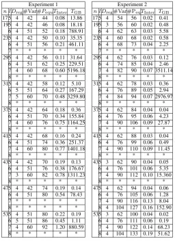
Table 1 compares Minisat with Gr¨obner basis methods (experiment 2) form= 4. The main observation of this experiment is we can handle larger values oflwith Minisat in reasonable amount of time than Gr¨obner basis methods. But the process has to be repeated 1/Psucc times on average, as the probability of finding a relation is decreased byPsucc. We also observe that the memory used by Minisat is much lower than that of the Gr¨obner basis algorithm. We do not report experiments using Gr¨obner basis method for values ofl >4
Table 1.Comparison of solving polynomial systems, when there exists a solution to the system, in experiment 2 using SAT solver (Minisat) versus Gr¨obner basis methods form= 4.#Varand#Pequare the number of variables and the number of polynomial equations respectively.Memis average memory used in megabytes by the SAT solver or Gr¨obner basis algorithm.#Clauses,
#Literals, andPsuccrepresent the average number of clauses, total number of literals, and the percentage of times Minisat halts with solutions within 200 seconds respectively.
Experiment 2 with SAT solver Minisat
n l#Var#Pequ#Clauses#LiteralsTInterTSATMemPsucc 173 54 59 46678 181077 0.35 7.90 5.98 94% 4 67 68 125793 485214 0.91 27.78 9.38 90% 193 54 61 55262 215371 0.37 3.95 6.07 93% 4 71 74 140894 543422 1.29 18.38 18.05 86% 233 54 65 61572 240611 0.39 1.53 7.60 87% 4 75 82 194929 760555 2.15 5.59 14.48 83% 5 88 91 394759 1538560 4.57 55.69 20.28 64% 294 77 90 221828 868619 3.01 7.23 19.05 87% 5 96 105 572371 2242363 9.95 39.41 32.87 67% 6 109 114 855653 3345987 21.23 15.87 43.07 23% 7 118 119 1063496 4148642 36.97 26.34133.13 14% 314 77 92 284748 1120243 3.14 17.12 20.52 62% 5 98 109 597946 2345641 11.80 33.48 45.71 57% 6 113 120 892727 3489075 26.23 16.45118.95 12% 7 122 125 1307319 5117181 44.77 21.98148.95 8% 374 77 98 329906 1300801 3.41 26.12 29.97 59%
5 100 117 755621 2977220 13.58 48.19 50.97 40% 6 119 132 1269801 4986682 41.81 42.85108.41 11% 7 134 143 1871867 7350251 94.28 40.15169.54 6% 414 77 102 317272 1250206 3.08 19.28 27.59 68%
5 100 121 797898 3146261 15.71 27.14 49.34 65% 6 123 140 1353046 5326370 65.25 31.69 89.71 13% 434 77 104 374011 1477192 2.97 17.77 28.52 68% 5 100 123 825834 3258080 13.85 29.60 54.83 52% 474 77 108 350077 1381458 3.18 11.40 29.93 59% 5 100 127 836711 3301478 14.25 27.56 61.55 43% 534 77 114 439265 1738168 11.02 27.88 32.35 75% 5 100 133 948366 3748119 14.68 34.22 64.09 62% 6 123 152 1821557 7200341 49.59 41.55123.38 11% 7 146 171 2930296 11570343 192.2067.27181.20 4%
Experiment 2 with Gr¨obner basis:F4 n l#Var#PequTInterTGB Mem
173 54 59 0.29 0.29 67.24 4 67 68 0.92 51.79 335.94 193 54 61 0.33 0.39 67.24
4 71 74 1.53 33.96 400.17 233 54 65 0.26 0.31 67.24
4 75 82 2.52 27.97 403.11 293 54 71 0.44 0.50 67.24
4 77 90 3.19 35.04 503.87 313 54 73 0.44 0.58 67.24
4 77 92 3.24 9.03 302.35 373 54 79 0.36 0.43 67.24
4 77 98 3.34 9.07 335.94 413 54 83 0.40 0.54 67.24
4 77 102 3.39 17.19 382.33 433 54 85 0.43 0.53 67.24
4 77 104 3.44 9.09 383.65 473 54 89 0.50 0.65 67.24
4 77 108 3.47 9.59 431.35 533 54 95 0.33 0.40 67.24
Table 2 compares experiment 1 and experiment 2 in the casem= 3. Gr¨obner basis methods are used in both cases. Timings are averages from 100 trials except for values ofTGB+TInter >200seconds, in this case they are single instances.
Experiments in [19] are limited to the casem= 3andl∈ {3,4,5,6}for prime degree extensions
n∈ {17,19,23,29,31,37,41,43,47,53}.
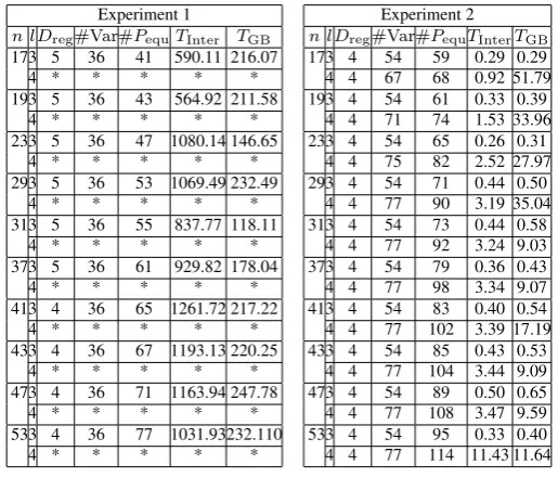
This is due to high running times and large memory requirements, even for small parameter sizes. As shown in Table 2, we repeated these experiments. Exploiting greater symmetry (in this case experiment 2) is seen to reduce the computational costs. Indeed, we can go up tol= 8with reasonable running time for somen, which is further than [19]. The degree of regularity stays≤4in both cases.
Table 2.Comparison of solving our systems of equations, having a solution, using Gr¨obner basis methods in experiment 1 and experiment 2 form = 3. Notation is as above. ’*’ indicates that the time to complete the experiment exceeded our patience threshold.
Experiment 1
n l Dreg#Var#PequTInter TGB
17 5 4 42 44 0.08 13.86 195 4 42 46 0.08 18.18 6 4 51 52 0.18 788.91 235 4 42 50 0.10 35.35
6 4 51 56 0.21 461.11
7 * * * * *
295 4 42 56 0.11 31.64 6 4 51 62 0.25 229.51 7 4 60 68 0.60 5196.18
8 * * * * *
315 4 42 58 0.12 5.10 6 5 51 64 0.27 167.29 7 5 60 70 0.48 3259.80
8 * * * * *
375 4 42 64 0.18 0.36 6 4 51 70 0.34 155.84 7 4 60 76 0.75 1164.25
8 * * * * *
415 4 42 68 0.16 0.24 6 4 51 74 0.36 251.37 7 4 60 80 0.77 1401.18
8 * * * * *
435 4 42 70 0.19 0.13 6 4 51 76 0.38 176.67 7 3 60 82 0.78 1311.23
8 * * * * *
475 4 42 74 0.19 0.14 6 4 51 80 0.54 78.43
7 * * * * *
8 * * * * *
535 4 51 80 0.22 0.19 6 5 51 86 0.45 1.11 7 4 60 92 1.20 880.59
8 * * * * *
Experiment 2
n l Dreg#Var#PeqTInter TGB
17 5 4 54 56 0.02 0.41 195 3 56 60 0.02 0.48 6 4 62 63 0.03 5.58 235 4 60 68 0.02 0.58 6 4 68 73 0.04 2.25
7 * * * * *
295 4 62 76 0.03 0.12 6 4 74 85 0.04 2.46 7 4 82 90 0.07 3511.14
8 * * * * *
315 4 62 78 0.03 0.36 6 4 76 89 0.05 2.94 7 4 84 94 0.07 2976.97
8 * * * * *
375 4 62 84 0.04 0.04 6 4 76 95 0.06 4.23 7 4 90 106 0.09 27.87
8 * * * * *
415 4 62 88 0.03 0.04 6 4 76 99 0.06 0.49 7 4 90 110 0.09 11.45
8 * * * * *
435 3 62 90 0.04 0.05 6 4 76 101 0.06 5.35 7 4 90 112 0.10 15.360
8 * * * * *
475 4 62 94 0.04 0.06 6 4 76 105 0.06 1.28 7 4 90 116 0.13 8.04 8 4 104 127 0.16 152.90 535 3 62 100 0.04 0.02
6 4 76 111 0.06 0.19 7 4 90 122 0.14 68.23 8 4 104 133 0.19 51.62
of regularity form = 4, stated in [25], ism2 + 1 = 17. The table shows that our choice of coordinates makes the casem= 4much more feasible.
Table 3.Comparison of solving our systems of equations, having a solution, using Gr¨obner basis methods in experiment 1 and experiment 2 form= 4. Notation is as above. The second tabular column already appeared in Table 1.
Experiment 1
n l Dreg#Var#PequTInter TGB
173 5 36 41 590.11 216.07
4 * * * * *
193 5 36 43 564.92 211.58
4 * * * * *
233 5 36 47 1080.14 146.65
4 * * * * *
293 5 36 53 1069.49 232.49
4 * * * * *
313 5 36 55 837.77 118.11
4 * * * * *
373 5 36 61 929.82 178.04
4 * * * * *
413 4 36 65 1261.72 217.22
4 * * * * *
433 4 36 67 1193.13 220.25
4 * * * * *
473 4 36 71 1163.94 247.78
4 * * * * *
533 4 36 77 1031.93232.110
4 * * * * *
Experiment 2
n l Dreg#Var#PequTInterTGB
173 4 54 59 0.29 0.29 4 4 67 68 0.92 51.79 193 4 54 61 0.33 0.39
4 4 71 74 1.53 33.96 233 4 54 65 0.26 0.31
4 4 75 82 2.52 27.97 293 4 54 71 0.44 0.50
4 4 77 90 3.19 35.04 313 4 54 73 0.44 0.58
4 4 77 92 3.24 9.03 373 4 54 79 0.36 0.43 4 4 77 98 3.34 9.07 413 4 54 83 0.40 0.54 4 4 77 102 3.39 17.19 433 4 54 85 0.43 0.53
4 4 77 104 3.44 9.09 473 4 54 89 0.50 0.65 4 4 77 108 3.47 9.59 533 4 54 95 0.33 0.40 4 4 77 114 11.43 11.64
Our idea of symmetry breaking (experiment 3) is investigated in Table 4 for the casem = 3. Some of the numbers in the second tabular column already appeared in Table 2. Recall that the relation probability is increased by a factor3! = 6in this case, so one should multiply the timings in the right hand column by
(m−1)! = 2to compare overall algorithm speeds. The experiments are not fully conclusive (and there are a few “outlier” values that should be ignored), but they suggest that symmetry-breaking can give a speedup in many cases whennis large.
For larger values ofn, the degree of regularityDreg is often 3 when using symmetry-breaking while it is 4 for most values in experiment 2. The reason for this is unclear, but we believe that the performance we observe is partially explained by the fact that the degree of regularity stayed at 3 asngrows.
7 Conclusions
We have suggested that binary Edwards curves are most suitable for obtaining coordinates invariant under the action of a relatively large group. Faug`ere et al [12] studied Edwards curves in the non-binary case and showed how the symmetries can be used to speed-up point decomposition. We show that these ideas are equally applicable in the binary case. For largeq and small none would get the same result as in [12]: that the FGLM complexity is reduced by a factor of2m−1. We have studied small q and large (prime)n
and shown that one can get overdetermined systems and that the use of symmetries reduces the degree of regularity.
Table 4.Comparison of solving our systems of equations using Gr¨obner basis methods having a solution in experiment 3 and experiment 2 whenm = 3. Notation is as in Table 1. For a fair comparison, the timings in the right hand column should be doubled.
Experiment 3
n l Dreg#Var#PequTInter TGB 375 3 68 90 0.04 0.25 6 4 80 99 0.07 5.67
7 * * * * *
415 4 68 94 0.05 0.39 6 3 80 103 0.07 4.55 7 4 93 113 0.11 1905.21 435 4 68 96 0.05 0.21
6 4 80 105 0.08 4.83 7 3 94 116 0.12 100.75 475 4 68 100 0.05 0.17
6 3 80 109 0.08 3.88 7 3 94 120 0.11 57.61 535 3 68 106 0.06 0.08
6 4 80 115 0.09 12.75 7 3 94 126 0.14 11.38 595 4 68 112 0.06 0.05
6 4 80 121 0.10 0.59 7 4 94 132 0.16 13.60 615 4 68 114 0.06 0.04
6 4 80 123 0.11 0.46 7 4 94 134 0.16 8.61 675 3 68 120 0.07 0.02 6 3 80 129 0.11 0.17 7 4 94 140 0.16 121.33 715 3 68 124 0.07 0.02
6 3 80 133 0.12 0.12 7 4 94 144 0.18 2.06 735 3 68 126 0.08 0.02 6 3 80 135 0.12 0.11 7 4 94 146 0.18 1.47 795 3 68 132 0.08 0.02 6 4 80 141 0.12 0.07 7 4 94 152 0.19 0.62 835 3 68 136 0.08 0.02 6 4 80 145 0.13 0.04 7 3 94 156 0.21 0.29 895 3 68 142 0.09 0.02 6 3 80 151 0.14 0.03 7 3 94 162 0.21 0.17 975 3 68 150 0.09 0.02 6 3 80 159 0.14 0.03 7 4 94 170 0.22 0.10
Experiment 2
n l Dreg#Var#PequTInter TGB 375 4 62 84 0.04 0.04 6 4 76 95 0.06 4.23 7 4 90 106 0.09 27.87 415 4 62 88 0.03 0.04
6 4 76 99 0.06 0.49 7 4 90 110 0.09 11.45 435 3 62 90 0.04 0.05
6 4 76 101 0.06 5.35 7 4 90 112 0.10 15.360 475 4 62 94 0.04 0.06
6 4 76 105 0.06 1.28 7 4 90 116 0.13 8.04 535 3 62 100 0.04 0.02 6 4 76 111 0.06 0.19 7 4 90 122 0.14 68.23 595 4 62 106 0.04 0.02
SAT solvers often work better than Gr¨obner methods, especially in the case when the system of equations has a solution with low hamming weight supported mainly on the lower bits. They are non-deterministic and the running time varies widely depending on the inputs, including the curve parameter. Unfortunately, most of the time SAT solvers are slow (for example, because the system of equations does not have any solutions). We suggest an early abort strategy that may still make SAT solvers a useful approach.
We conclude by analysing whether these algorithms are likely to be effective for ECDLP instances in
E(F2n)whenn > 100. The best we can seem to hope for in practice ism = 4andl ≤ 10. Note that the linear algebra cost is negligible for such parameters. Since the probability of a relation is roughly2lm/2n, so the number of trials (i.e., executions of polynomial system solving) needed to find a relation is at least
2n/2ml ≥2n−40 ≥√2n. Since solving a system of equations is much slower than a group operation, we conclude that our methods are worse than Pollard rho. This is true even in the case of static-Diffie-Hellman, when only one relation is required to be found. Hence, we conclude that elliptic curves in characteristic 2 are safe against these sorts of attacks for the moment, though one of course has to be careful of other “Weil descent” attacks in this case, such as the Gaudry-Hess-Smart approach [15].
Acknowledgements
We thank Claus Diem, Christophe Petit and the anonymous referees for their helpful comments.
References
1. Daniel J. Bernstein, Tanja Lange and Reza Rezaeian Farashahi, Binary Edwards Curves, in E. Oswald and P. Rohatgi (eds.), CHES 2008, Springer LNCS 5154 (2008) 244–265.
2. Luk Bettale, Jean-Charles Faug`ere and Ludovic Perret, Hybrid approach for solving multivariate systems over finite fields, J. Math. Crypt.3(2009) 177–197.
3. Daniel R. L. Brown and Robert P. Gallant, The Static Diffie-Hellman Problem, IACR Cryptology ePrint Archive 2004/306 (2004)
4. Nicolas T. Courtois and Gregory V. Bard, Algebraic Cryptanalysis of the Data Encryption Standard, in S. D. Galbraith (ed.), IMA Int. Conf. Cryptography and Coding, Springer LNCS 4887 (2007) 152–169.
5. Claus Diem, On the discrete logarithm problem in elliptic curves over non-prime finite fields, Lecture at ECC 2004, 2004. 6. Claus Diem, On the discrete logarithm problem in class groups of curves, Mathematics of Computation,80(2011) 443-475 7. Claus Diem, On the discrete logarithm problem in elliptic curves, Compositio Math.147, No. 1 (2011) 75–104.
8. Claus Diem, On the discrete logarithm problem in elliptic curves II, Algebra and Number Theory,7, No. 6 (2013) 1281–1323. 9. Iwan M. Duursma, Pierrick Gaudry and Francois Morain, Speeding up the discrete logarithm computation on curves with
automorphisms, in K.Y. Lam, E. Okamoto and C. Xing (eds.), ASIACRYPT 1999, Springer LNCS 1716 (1999) 103–121. 10. Niklas E´en and Niklas S¨orensson, The Minisat Page,http://www.minisat.se/
11. Jean-Charles Faug`ere, Ludovic Perret, Christophe Petit and Gu´ena¨el Renault, Improving the Complexity of Index Calculus Algorithms in Elliptic Curves over Binary Fields, in D. Pointcheval and T. Johansson (eds.), EUROCRYPT 2012, Springer LNCS 7237 (2012) 27–44.
12. Jean-Charles Faug`ere, Pierrick Gaudry, Louise Huot and Gu´ena¨el Renault, Using Symmetries in the Index Calculus for Elliptic Curves Discrete Logarithm, to appear in Journal of Cryptology (2014). doi:10.1007/s00145-013-9158-5
13. Jean-Charles Faug`ere, Louise Huot, Antoine Joux, Gu´ena¨el Renault and Vanessa Vitse, Symmetrized summation polynomials: Using small order torsion points to speed up elliptic curve index calculus, in P. Q. Nguyen and E. Oswald (eds.), EUROCRYPT 2014, Springer LNCS 8441 (2014) 40-57.
14. Jean-Charles Faug`ere, P. Gianni, D. Lazard, and T. Mora. Efficient Computation of zero-dimensional Gr¨obner bases by change of ordering, Journal of Symbolic Computation,16, No. 4 (1993) 329–344.
15. Pierrick Gaudry, Florian Hess, and Nigel P. Smart, Constructive and destructive facets of Weil descent on elliptic curves, J. Crypt.,15, no. 1 (2002) 19–46.
16. Pierrick Gaudry, Index calculus for abelian varieties of small dimension and the elliptic curve discrete logarithm problem, Journal of Symbolic Computation,44, no. 12 (2009) 1690–1702.
18. Robert Granger, On the Static Diffie-Hellman Problem on Elliptic Curves over Extension Fields, in M. Abe (ed.), ASIACRYPT 2010, Springer LNCS 6477 (2010) 283–302.
19. Yun-Ju Huang, Christophe Petit, Naoyuki Shinohara and Tsuyoshi Takagi, Improvement of Faug`ere et al.’s Method to Solve ECDLP, in K. Sakiyama and M. Terada (eds.), IWSEC 2013, Springer LNCS 8231 (2013) 115–132.
20. Antoine Joux, Reynald Lercier, David Naccache and Emmanuel Thom´e, Oracle-Assisted Static Diffie-Hellman Is Easier Than Discrete Logarithms, in M. G. Parker (ed.), IMA Int. Conf. Cryptography and Coding, Springer LNCS 5921 (2009) 351–367. 21. Antoine Joux and Vanessa Vitse, Cover and Decomposition Index Calculus on Elliptic Curves Made Practical - Application to a Previously Unreachable Curve overFp6, in D. Pointcheval and T. Johansson (eds.), EUROCRYPT 2012, Springer LNCS 7237 (2012) 9–26.
22. Antoine Joux and Vanessa Vitse, Elliptic Curve Discrete Logarithm Problem over Small Degree Extension Fields - Application to the Static Diffie-Hellman Problem onE(Fq5), J. Cryptology,26, no. 1 (2013) 119–143.
23. Neal Koblitz and Alfred Menezes, Another look at non-standard discrete logarithm and Diffie-Hellman problems, J. Mathe-matical Cryptology,2, No. 4 (2008) 311–326.
24. Cameron McDonald, Chris Charnes and Josef Pieprzyk, Attacking Bivium with MiniSat, ECRYPT Stream Cipher Project, Report 2007/040 (2007).
25. Christophe Petit and Jean-Jacques Quisquater, On Polynomial Systems Arising from a Weil Descent, in X. Wang and K. Sako (eds.), ASIACRYPT 2012, Springer LNCS 7658 (2012) 451–466.
26. Michael Shantz and Edlyn Teske, Solving the Elliptic Curve Discrete Logarithm Problem Using Semaev Polynomials, Weil Descent and Gr¨obner Basis Methods - An Experimental Study, in M. Fischlin and S. Katzenbeisser (eds.), Number Theory and Cryptography - Papers in Honor of Johannes Buchmann on the Occasion of His 60th Birthday, Springer LNCS 8260 (2013) 94–107.
27. Igor A. Semaev, Summation polynomials and the discrete logarithm problem on elliptic curves, Cryptology ePrint Archive, Report 2004/031, 2004.
28. Niklas S¨orensson and Niklas E´en, MiniSat - A SAT Solver with Conflict-Clause Minimization. Proc. Theory and Applications of Satisfiability Testing (SAT 05) 2005.
29. Niklas S¨orensson and Niklas E´en, Minisat 2.1 and minisat++ 1.0, SAT race 2008 editions, SAT (2008) 31–32.
30. Bo-Yin and Jiun-Ming Chen, Theoretical analysis of XL over small fields, in H. Wang, J. Pieprzyk and V. Varadharajan (eds.), ACISP, Springer LNCS 3108 (2004) 277–288.
31. Bo-Yin Yang, Jiun-Ming Chen and Nicolas Courtois, On asymptotic security estimates in XL and gr¨obner bases-related alge-braic cryptanalysis, in J. Lopez, S. Qing and E. Okamoto (eds.), ICICS, Springer LNCS 3269 (2004) 401–413.