A specific large-scale pressure gradient forcing for computation of realistic
13D wind fields over a canopy at stand scale
23 4
François Pimont
1, Jean-Luc Dupuy
1, Rodman Linn
2, Jeremy Sauer
2 56
1 INRA, Unité d’Ecologie des Forêts Méditerranéennes, Equipe de Prévention des Incendies
7
de Forêt, UR 629, F-84914, Avignon, France.
8
2 Los Alamos National Laboratory MS: D401, Los Alamos, New Mexico, 87544, USA.
9 10
Corresponding author François Pimont
11
Email: [email protected]
12 13
Abstract
1415
Turbulent flows over and within forest canopies have recently been modeled with success
16
using Large Eddy Simulations (LES). Validation exercises against experimental data suggest
17
that models can be applied with a high degree of confidence for many applications,
18
mechanical and physiological plant/atmosphere interaction analysis, seed or pollen dispersal,
19
wildfire spread and firebrand transport, or investigation of causes of eddy-covariance
20
technique bias. Long distances required for shear-induced turbulence to equilibrate, result in
21
the widespread use of cyclic boundary conditions in LES atmospheric boundary layer studies.
22
Vegetation drag dissipates air momentum in the atmosphere, but equilibrium is often achieved
23
through compensatory momentum source, supplied by macro-scale pressure gradient forcing.
24
Unfortunately, both classical Ekman balance or simple spatially-constant pressure gradient
25
techniques for implementing this forcing have major drawbacks in the context of cyclic
26
boundary conditions for the applications listed above. Among them, it is difficult to specify
27
aspects of the mean velocity profile such as a specific desired wind velocity and direction at a
28
reference height. In the present paper, we propose a new technique for capturing the effects of
29
a large-scale pressure gradient force (LSPGF) that can be used at stand scale and enables
30
simulation of realistic and specifiable wind fields. Several variants of this LSPGF are
31
developed and analyzed here and validated against experimental data. Although this LSPGF
32
technique is developed in the context of HIGRAD/FIRETEC wildfire simulations, LSPGF
33
can be used for any LES wind modeling application aimed at generating detailed stand-scale
34
wind fields with resolved turbulence and shear profiles consistent with vegetation structure in
35
the boundary layer.
36 37
Keyword Ekman balance - Forest canopy – Large-eddy simulation – Large-scale pressure
38
gradient - Streaks
39 40 41
1 Introduction
4243
Turbulent flows over forest canopy and forest gaps have been studied in wind-tunnel, field
44
and numerical experiments (Finningan 2000), leading to a good understanding of turbulence
45
development mechanisms and a better knowledge of turbulence structures in homogeneous
46
canopies and at forest edges. A variety of numerical models are now used to simulate wind
47
fields with a reasonable degree of accuracy. Among the different techniques used to simulate
wind flows, one of the most fruitful approaches is the Large Eddy Simulation (LES), that
49
enables explicit computation of the turbulent structures larger than grid size (Shaw and
50
Schumann 1992; Kanda and Hino 1994; Patton et al. 1998; Su et al. 1998; Watanabe 2004;
51
Yang et al. 2006; Dupont and Brunet 2008a; Pimont et al. 2009). This technique can be
52
applied to a wide variety of investigations. First, simulations can be analyzed in detail to
53
understand the mechanisms associated with interactions between canopy and wind flow
54
(Dwyer et al. 1997; Dupont and Brunet 2008b; Dupont et al. 2010) or to determine the spatial
55
extent and other important properties of transition zones in heterogeneous canopies (Yang et
56
al. 2006; Pimont et al. 2011; Dupont et al. 2011). These modeled wind flows that are
57
consistent with canopy structure can also be used to simulate seed (Nathan et al. 2005) and
58
pollen (Chamecki et al. 2009) dispersal, to prescribe the computational domain boundaries for
59
physics-based wildfire behavior modeling (Pimont et al. 2011) or firebrand transport (Koo et
60
al. 2012). They can help explain some of the discrepancies observed when eddy-covariance
61
techniques are used for the measurement of carbon exchange between the biosphere and the
62
atmosphere (Kanda et al. 2004).
63 64
The development of resolved canopy-shear-induced turbulence requires fetch distances much
65
greater than the desirable domain size for the studies described above (~hundreds of metres).
66
Cyclic boundary conditions allow the modeler to side-step explicit representation of vast
67
distances (thereby reducing computational resource requirements) for turbulent boundary
68
layer development by making the assumption that the fetch of the development is statistically
69
homogeneous. A cyclic domain essentially serves as a Lagrangian window that moves
70
downwind as the shear profile develops and allows for the economical development of the
71
turbulence fields. Unfortunately, the current use of cyclic boundary conditions for extended
72
simulation periods has drawbacks, detailed below.
73 74
The investigation of phenomenology in the context of specific conditions requires setting
75
some characteristics of the mean wind profile such as the wind velocity and direction at a
76
given height (e.g, reproducing fire experiments, see Linn et al. (2012), particle or scalar
77
transport), which is not trivial with cyclic boundary conditions. Vegetation drag acts as a
78
momentum sink in the lower part of the boundary layer. Without the presence of a mesoscale
79
pressure force to counterbalance this sink, the mean wind velocity tends to decay over time
80
when no momentum source is provided at the domain top. In scenarios where a source of
81
momentum is provided by a top-boundary absorbing layer (i.e. a Rayleigh damping layer), it
82
tends to distort the shear profile and results in vertical velocity profiles resembling those
83
found in a turbulent Couette flow in the upper part of the domain, which is not realistic for the
84
atmosphere (Watanabe, 2004; Pimont et al. 2009). Setting a given wind velocity at a given
85
height is all the more complex because the top boundary winds have no physical relevance
86
(Pimont et al. 2011).
87 88
A second approach for wind profile convergence is based on the Ekman balance (Holton and
89
Hakim 2012), in which a mesoscale pressure gradient acts in combination with the Coriolis
90
force, topography and soil or vegetation friction. The geostrophic layer is the zone of the
91
planetary boundary layer (PBL) where shear induced by the ground is negligible, so that
92
winds are in geostrophic balance between pressure and Coriolis terms. The wind direction is
93
normal to the mesoscale pressure gradient. Lower in the atmosphere and especially near the
94
ground, the wind is not normal to pressure gradient, so that the pressure gradient has a
non-95
zero component along the mean wind direction that compensates for the
surface-friction-96
induced wind-velocity decay. This balance can be implemented in computations with a
97
directional shift in wind direction from the top of the domain to the ground (Moeng and
Sullivan 1994; Dupont et al. 2011). Similarly to the scenario where no pressure gradient is
99
used, the Ekman balance yields a lack of control over wind speed and direction close to the
100
canopy, since those depend on the geostrophic wind magnitude and direction and vegetation
101
characteristics. Moreover, a strong wind directional shift between canopy top and canopy
102
bottom occurs in simulations and this swing can be overestimated compared to experimental
103
data (Dupont et al. 2011). Additionally, the significant wind rotation with height complicates
104
the interpretation of the cyclic domain since winds at different heights, moving in directions,
105
travel different distances as they traverse a domain. The use of the Ekman balance is thus not
106
satisfactory in many situations. A third approach commonly reported in the literature to
107
ensure wind profile convergence is based on the notion that a pressure gradient force
108
compensates for the drag force of surface roughness elements to produce stationary velocity
109
and turbulence profiles.
110 111
With this in mind, a large-scale pressure gradient field could be implicitly derived from wind
112
decay (or acceleration) of the average winds within the domain over time to ensure a constant
113
integrated mass flux across the domain. In this case, the Coriolis force is not involved.
114
Several authors implemented such an adaptive forcing for studying the interaction between
115
wind and canopy using an assumption of constant pressure gradient over the height of the
116
domain (Shaw and Shumann 1992; Dwyer et al. 1997; Patton 1997; Patton et al. 1998) or in
117
the upper part only (Su et al. 1998; Yang et al. 2006). Again, there is no control on the wind
118
velocity at a given height. Another drawback of this approach was that domain heights were
119
limited to 3 to 6 times the height of the canopy, because of computational limitation, but also
120
because the assumption of a spatially-constant pressure gradient force at higher elevations is
121
not realistic. In the context of wildfires, vertical domain extents of several hundreds to several
122
thousands of meters are required to appropriately capture the interaction between the plume
123
and atmosphere. In other applications such as particle dispersal analysis, significant domain
124
heights are also often required to allow for particle lofting, therefore a restriction imposed on
125
vertical domain extent is prohibitive to many studies. Another limitation of this approach was
126
mentioned by Patton (1997), who reported an unusually large forcing due to limited domain
127
height and overestimations of the mean streamwise velocity. Finally, this spatially-constant
128
pressure gradient approach requires a free-slip top boundary, whereas atmospheric models
129
such as those used by Pimont et al. (2009) or Dupont and Brunet (2008a), often use Rayleigh
130
damping layers at the top of the domain to absorb upward-propagating wave disturbances and
131
eliminate wave reflection at the top-boundary, again limiting the applicability of this
132
approach.
133 134
Finally, cyclic-boundary conditions induced the development of large streamwise vortices
135
called “streaks”, that have sometimes been reported as being unrealistically large and
136
persistent. In nature, such structures appear under neutral or stable conditions in the presence
137
of significant surface layer roughness, such as heterogeneous canopies (Drobinski and Foster
138
2003). The observed streak structure size can be as large as several hundreds of meters
139
(Deardorff 1980; Moeng and Sullivan 1994; Lin et al. 1996; Drobinski and Foster 2003).
140
They normally build, evolve and disappear over periods of several tens of minutes (Foster
141
1997; Lin et al. 1996; Drobinski et al. 1998; Drobinski and Foster 2003). Some authors
142
reported streaks occurring in LES simulations (Moeng and Sullivan 1994; Watanabe 2004;
143
Pimont et al. 2011). Pimont et al. (2011) observed that on relatively small computational
144
domains (less than 300 m in width) with no representation of a large-scale pressure gradient
145
force, they maintain over time, do not evolve and have unrealistically high magnitude. Those
146
unrealistic structures are clearly a significant limitation for most of the application described
147
above.
149
This manuscript presents a new implementation of a specific large-scale pressure gradient
150
force formulation designed to enable the computation of realistic wind fields for subsequent
151
use in stand scale atmospheric phenomena investigation, such as coupled fire/atmosphere
152
simulations. This pressure gradient approach is designed to avoid the drawbacks mentioned
153
above and to be amenable to studies targeting a prescribed wind velocity at a given height.
154 155 156
2 Model description
157158
2.1 HIGRAD/FIRETEC
159 160
The HIGRAD/FIRETEC model is the coupling between an atmospheric model (HIGRAD,
161
Reisner et al. 2000) and a combustion and heat transfer model (FIRETEC, Linn et al. 2005).
162
HIGRAD solves the compressible Navier-Stokes equations using the method of averages
163
(MOA). The MOA scheme combines and averages the advective tendency, buoyancy, local
164
pressure gradient, and Coriolis force terms of the momentum equations over several small
165
time steps on the order of a millisecond with a computationally inexpensive first-order
166
accurate scheme. Subsequently the combined and averaged forces along with averaged
167
advective velocities are used to calculate a larger time step evolution with a second order
168
accurate scheme in time and space yielding a numerical damping of sound waves and
169
effective relaxation of Courant condition within the model (see Reisner et al. 2000 for more
170
details). Turbulence and drag are represented as a part of the FIRETEC model and details are
171
described in Pimont et al. (2009). In the present paper, we test the implementation in
172
HIGRAD/FIRETEC of the specific large-scale pressure gradient forces (LSPGF) described in
173
Sect. 2.2.
174 175
2.2 Large-scale pressure gradient forces (
LSPGF
)
176 177
The aim of the following derivation is to develop a new methodology for capturing the effects
178
of large-scale pressure gradient forces, that combines the benefits of the Ekman balance and
179
spatially-constant pressure gradient force described in Sect. 1. This approach is intended to
180
overcome the known drawbacks of these previous approaches applied, namely the lack of
181
control of wind speed and direction close to the canopy, as well as the development of
182
unrealistic “streaks”.
183 184
For a geostrophic wind aligned with the x-axis and of magnitude Ug (Fig. 1), the effect of the
185
mesoscale pressure gradient and Coriolis force terms in the momentum equation can be
186
expressed as forces: fv and in the u and v momentum equations (with u and v the
187
zonal and meridional components of wind velocity respectively), with f being the Coriolis
188
parameter (Dupont et al. 2011, for example) and
€
ρ the air density. A consequence of those
189
forces is the rotation of the direction of the flow as one descends from the upper geostrophic
190
layer to the ground. The effect of the Coriolis and large scale pressure gradient forces on the
191
evolution of the horizontal wind velocity magnitude, , at a given height with time
192
can be derived from the free atmosphere equations for u and v:
193
(1)
194
The physical meaning of this expression is that the balance between Coriolis and large-scale
196
pressure gradient at a given altitude both rotates flow direction and changes the
velocity-197
magnitude profile due to an effective induced pressure gradient of magnitude
198
(2)
199
where s is the direction of the flow at this altitude. This force per unit mass is the projection
200
of (pressure gradient force in the y-direction) in the direction of the mean wind
201
at a given height, because is the sine of wind direction angle and the
202
geostrophic wind (Fig. 1).
203
204
Fig. 1 205
Projection of the geostrophic on the wind direction
206 207
The specific formulation for the effects large-scale pressure gradient forces presented here is
208
intended to approximate the streamwise component of the combined Coriolis force and the
209
mesoscale pressure gradient force (Eq. 2), so that it mimics the stable Ekman balance, but
210
without the directional change effects. The absence of directional changes was motivated by
211
the problem associated with direction control and significant challenges with use of cyclic
212
boundary conditions as described above. The consequences of this point will be discussed
213
later.
214
In Eq. 2, v
u2 +v2 can be approximated in using the Ekman spiral (Holton and Hakim 2012, 215
p 267),
216
(3)
217
(4)
218 219
with and K being an eddy diffusivity.
220 221
For a geostrophic wind Ug along the x-axis, the effect of the large scale pressure gradient force
222
can be written,
223
(5)
224
with (6)
225
226
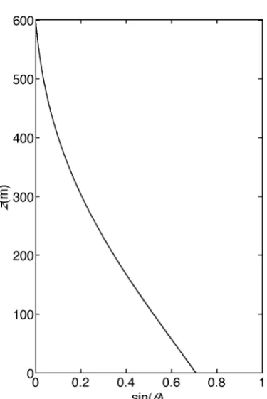
A representation of is shown in Fig. 2, assuming a geostrophic layer of 600 m
227
γ =π / 600
(
)
.
229
230
Fig. 2 231
sinθ(z) profile (Eq. 6) using Ekman’s assumptions and
232 233
Beyond the vertical rotation and velocity enhancement, the influence of mesoscale pressure
234
gradient and Coriolis forces also ensures a stable equilibrium of mass flow (Ekman balance).
235
Assuming that ueq(z) and veq(z) are the solution of the u and v velocity profiles in the context of
236
the the Ekman balance. When v(z) is smaller than the balance veq(z), the forcing on u velocity
237
by fv will be smaller than the one at the Ekman balance ueq, so that the forcing on v velocity
238
f(Ug-u) will be greater than the one at the balance veq. The combination of mesoscale pressure
239
gradient and Coriolis forces act in combination to steer the u and v velocity profiles towards
240
convergence in a stable Ekman balance.
241 242
In order to ensure convergence of the momentum, a dynamic adjustment of the pressure force
243
described in Eq. 2 is achieved through adjustment of the parameter f. f was dynamically
244
updated, with the rule described below:
245
LetM(t)= ρu dx dy dz
x,y,z
∫∫∫
the integral of the momentum over the domain at a given time t246
and Meq= ρueqdx dy dz x,y,z
∫∫∫
at the equilibrium state. Assuming a constant value of the f247
parameter between t-Δt and t+Δt, M(t+Δt) can be estimated as 2M(t)-M(t-Δt). The
248
modification of f required to set M(t) to Meq can thus be derived from the integration over time
249
and space of the momentum equation:
250
(7)
251
so that,
(8)
253
where lx and ly are the horizontal length of the domain in the x and y direction respectively. Meq
254
can then be estimated from an initial empirical wind profile (see Appendix A).
255 256
Equation 8 provides a rule to modify the value of f every Δt, so that the integrated momentum
257
will be conserved over the duration of the simulation by applying a force that mimics the
258
vertical force distribution resulting from geostrophic LSGF and Coriolis force. The
259
application of this force in the streamwise direction alleviates the complications associated
260
with the swing in velocity direction with height when using cyclic boundary conditions. The
261
time interval at which f should be updated (Δt) was derived from an analysis of the speed of
262
decay of the integrated momentum when no pressure gradient was used. The LSPGF is a very
263
small forcing that affects the integrated momentum at a slow rate, so that Δt is much bigger
264
than the computational time step. This version of LSPGF will be hereafter referred to as
265
LSPGF1, LSPGF0 being the case with no pressure gradient force (Table 1).
266 267
The LSPGF scheme described above is based on the integration of the momentum over the
268
whole domain. It is possible to perform the same derivation focusing on a 2D horizontal slice
269
at a reference height zref to define . In this context, can be
270
defined as , with uref the mean target velocity at reference height zref. We can update the
271
value of f, using,
272
(9)
273
This scheme ensures convergence of the integrated momentum to
€
Meqzref
, so that uref
274
will be the balance velocity at height zref. This version of LSPGF will be hereafter referred to
275
as LSPGF2 (Table 1) and will be shown to have particular applicability when empirical
276
characterization of wind fields is based upon a mean velocity at a specified height.
277 278
The stable Ekman balance acts to limit streak magnitude. When a spatially-homogeneous
279
pressure gradient forcing is applied across a horizontal plane (e.g. classical spatially-constant
280
pressure gradient, LSPGF1, LSPGF2), one drawback of using cyclic boundary conditions is
281
the development of unusually strong and persistent “streaks” (streamwise vortices). These
282
streaks result in alternating lines of faster and slower streamwise flows above the canopy. The
283
mean flow will converge, but there is no mechanism to limit the development of streaks of
284
strong magnitude, apart from the lateral shear induced by the streaks. This single limiting
285
mechanism is insufficient to maintain appropriate streak strength. A third version of LSPGF,
286
hereafter referred to as LSPGF3 (Table 1) was developed to mimic the Ekman balance
287
horizontal stability, thereby providing an additional means of limiting the magnitude of
288
streaks in a physically relevant manner. Instead of having f constant at a given height, as for
289
LSPGF1 and LSPGF2, the momentum integration can be performed along streamwise lines
290
so that the value of M varies in the spanwise direction. For example, when the wind is aligned
291
with the x-axis, the integrated momentum can be computed for
292
every y. If the wind is faster in line y1, than in line y2, the will be greater than
293
, so that the pressure gradient update will be higher in line y1 than in line y2. Such a
294
rule requires that the integrals of the vegetation leaf-area density averaged in the x direction
are equal or at least similar for all y. This constraint suggests that not all vegetation
296
configurations can be directly simulated with LSPGF3. This point will be discussed later, as
297
well as a solution for the other scenarios. To avoid high-frequency spatial variations in
298
LSPGF forcing, an optional Gaussian filter in the y-direction with a footprint of about the size
299
of streaks (100 m) can be imposed to the forcing on f after the update described above for a
300
given z, but it has little effect on the final results. The implementation of this variant of
301
LSPGF is relatively straightforward when wind is aligned with the x or y-axis. When the wind
302
is not aligned with domain axis, integrated momentum should be computed along the mean
303
wind direction as is developed in Appendix B.
304 305
Table 1 306
Description of the different large-scale pressure gradient forces (for a geostrophic wind ,
307
with the unit vector of the x-axis). zref is the reference height where velocity uref is targeted
308
is defined according to Eq. 6. lx, lyare horizontal extents of the domain along the x,
y-309
axis
310 311
Mode Pressure force Integrated momentum
LSPGF0 0 - -
LSPGF1
LSPGF2
LSPGF3
EKMAN fv and f(Ug-u) in x and y direction
- -
312 313
3 Numerical experiment
314315
3.1 Vegetation scenarios
316 317
Simulations were performed using HIGRAD/FIRETEC over four different canopies (Table
318
2). It should be noticed that canopy C4 was extrapolated from the wind tunnel study of
319
Raupach et al. (1987). This experimental set has already been used by several authors
320
(Dupont et al. 2008b; Pimont et al. 2009), because of the completeness of the wind statistic
321
data set. Additional details about these canopies and data collected in the field can be found in
322
the reference paper cited for each scenario.
323 324
Table 2 325
Description of the four canopy configurations used in the present study
326
Scenario Canopy type Reference Canopy height; LAI; structure
C1 Homogeneous,
maritime pine
Dupont et al. (2011) h = 22 m; LAI = 2 (+understorey 0.5); 512
m forest
C2 Forest edge,
maritime pine
Dupont et al. (2011) h = 22 m; LAI = 2(+understorey 0.5)/0.5
(forest/open); 200 m open/312 m forest
C3 Deciduous
forest
Shaw et al. (1988), Pimont et al. (2009)
h = 18 m; LAI = 2; 512 m forest
from wind
tunnel, forest
edge
et al. (2009) open/268 m forest
327
3.2 Numerical details
328 329
A 512 m ⋅ 512 m ⋅ 615 m domain was used for all runs except the one above canopy C4,
330
where a slightly longer domain was used to more accurately represent forest to open and open
331
to forest transitions (768 m). Horizontal resolution was uniformly 2 m, whereas vertical
332
resolution incorporates a cubic stretching with values from 1.5 m at the surface to 2.9 m
333
below the canopy increasing with height above ground to 50 m near domain top (41 vertical
334
cells). The initial wind velocities and geostrophic wind (wind at domain top cell center at z =
335
595 m) were set using empirical profiles described in Appendix A (using uini=6 m s-1 at 40 m).
336
These profiles are defined based on LAI and fuel height h in each stand. They use a log
337
profile above 2h and an exponential profile below h. The modeled scenario was run with a
338
time step dt = 0.002 s (small time step to account for pressure perturbation), with the method
339
of averages applied over 10 small time steps. For all runs, a drag coefficient C_d of 0.15 was
340
chosen. It should be noticed that Dupont et al. (2011) used a drag coefficient of 0.26 derived
341
from field measurements. A single value of drag coefficient for all numerical experiments was
342
chosen for simplicity and in light of past studies indicating the limited effect of this parameter
343
on normalized data (Pimont et al. 2009).
344 345
3.3 Set of simulations
346 347
Using canopy C1, the model was run without pressure gradient forcing (LSPGF0), and
348
subsequently with the three versions of LSPGF described above (LSPGF1, LSPGF2,
349
LSPGF3) with Δt = 200 s (update period of LSPGF) and finally with the classical Ekman
350
balance (EKMAN) approach. Using canopy C2, C3 and C4, four simulations were performed
351
with LSPGF3 and wind flow statistics were computed and plotted against experimental data
352
(Table 2) to evaluate the model skill. Canopy C2 was also used with three different initial
353
profiles and geostrophic winds using LSPGF3 (“FOREST”, “OPEN” and “FOREST+20%”)
354
to illustrate the sensitivity to those parameters. “FOREST” used the empirical profile from
355
Appendix A using the canopy zone parameters (h=22 m, LAI=2.5). “OPEN” used the
356
empirical profile from Appendix A using the open zone parameters (h = 0.5 m, LAI = 0.5). A
357
third profile referred later to as “FOREST+20%”, uses the same profile as “FOREST”, but
358
wind velocities were increased to 20 % above 300 m, so that the geostrophic wind was 20 %
359
higher. It should be noticed that the integrals of vegetation leaf area density along the x-axis
360
are equal for all y, so that LSPGF3 can be used in all scenarios.
361 362
Table 3 363
Description of the main characteristics of the simulated scenarios
364
Simulation Canopy type Pressure gradient Initial profile parameters (Appendix A):
uref = 6 m s-1; zref = 40 m
LSPGF0 C1 No h = 22 m; LAI = 2.5
LSPGF1 C1 LSPGF1 h = 22 m; LAI = 2.5
LSPGF2 C1 LSPGF2 h = 22 m; LAI = 2.5
LSPGF3 C1 LSPGF3 h = 22 m; LAI = 2.5
EKMAN C1 Mesoscale+Coriolis force h = 22 m; LAI = 2.5
C2 C2 LSPGF3 h = 22 m; LAI = 2.5
C3 C3 LSPGF3 h = 18 m; LAI = 2.0
FOREST C2 LSPGF3 h = 22 m; LAI = 2.5
OPEN C2 LSPGF3 h = 0.5 m; LAI = 0.5
FOREST+20% C2 LSPGF3 h = 22 m; LAI = 2.5
initial profile is increased by 20 % above 300 m 365 366
4 Results
367 3684.1 Comparison between no pressure gradient (
LSPGF0
),
LSPGF1
,
LSPGF2
,
369
LSPGF3
and classical Ekman balance (
EKMAN
) for canopy
C1
370371
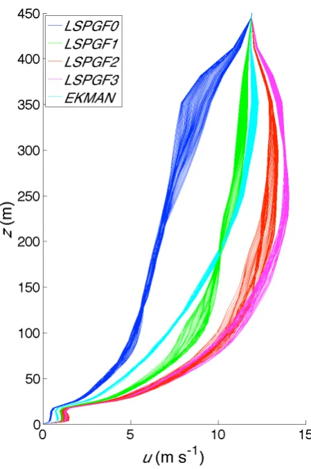
Figure 3 represents the evolution with time of mean velocity spatially averaged across the
372
domain for LSPGF0, LSPGF1, LSPGF2, LSPGF3 and EKMAN, at four reference heights
373
(3.88 m, 21.1 m, 40.0 m and 155 m). These simulations began with a spin-up period of 200 s,
374
during which the shear associated to drag induces a decay of wind velocity at the canopy top
375
(21.1 m) and the development of turbulence. Turbulence is fully developed after about 500 s,
376
as shown by the convergence of normalized turbulent kinetic energy (TKE) profiles computed
377
from resolved velocity fluctuations and modeled turbulent kinetic energy (not shown). In the
378
simulation without pressure gradient (LSPGF0), the wind velocity slowly declines at all
379
heights, resulting in an inappropriately low simulated velocity magnitude in the lower part of
380
the domain (2.8 m s-1 at 40 m). The convergence below 155 m takes about 3000 s and is
381
reached when the momentum source at the top of the domain is in equilibrium with the drag
382
force and turbulence dissipation. An analysis of the early part of the simulation shows that the
383
decay is about 5 % every 200 s. This is the justification for Δt (LSPGF update frequency) to
384
be chosen as every 200 s.
385 386
The Ekman balance (EKMAN) simulation converges quickly at each of the different heights,
387
as do simulations LSPGF1, LSPGF2 and LSPGF3. However, the four runs do not converge to
388
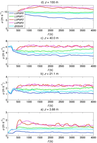
the same values. More generally, they converge to different profiles as illustrated in Fig. 4.
389
For each simulation, Figure 4 plots 50 different instantaneous profiles taken every 200 s
390
between 3000 and 4000 s and horizontally averaged. The decay of the wind speed in LSPGF0
391
is clearly visible in the upper part of the domain where the strong shear develops at the lower
392
boundary of the damping layer, as well as the convergence to a S-profile shape. This S-shape
393
in the LSPGF0 case where momentum is only fed by the geostrophic wind, may be viewed as
394
a limited slip Couette flow with strong mixing in the domain interior. Vertical turbulent
395
transport of momentum induced by the vegetation drag leads to a concave-up (instead of
396
linear) profile in the lower part of the domain above the vegetation. This convex profile is
397
counterbalanced by a concave-down region near the interface with the damping layer,
398
resulting in the S shape profile.
399 400
Considering the EKMAN and different LSPGF approaches, Fig. 4 illustrates that the profile
401
evolves only slightly over time, but in a limited range because the LSPGF simulations have a
402
forcing that adapts to drive a profile convergence. However the global shape of these profiles
403
are different in addition to producing significant variability in mean wind velocity at a 40 m
404
height, namely 5.1, 6.1, 6.1 and 3.8 m s-1 for LSPGF1, LSPGF2, LSPGF3, and EKMAN
405
respectively. The fact that the EKMAN case converges to 3.2 m s-1 illustrates that the
406
geostrophic wind value chosen for this computation using the wind profile described in
407
Appendix A, was too low to reach the target velocity of 6 m s-1 at 40 m. This result
408
demonstrates the challenge to set initial conditions (i.e. a geostrophic wind) targeting a given
fully-developed wind at a specified reference height, even when using a relatively
410
sophisticated estimation of the empirical profile described in Appendix A as initial condition.
411
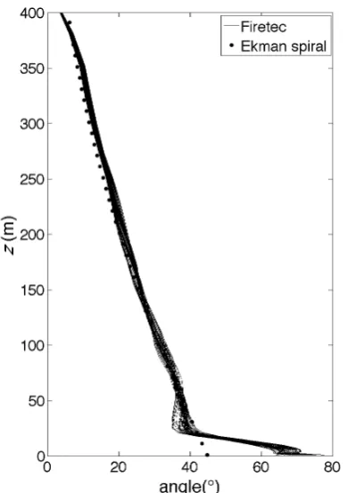
Figure 5 shows the angle between wind direction and geostrophic wind, as a function of
412
height when using the Ekman balance (EKMAN). The angle increases with distance
413
downward from the bottom of the damper (at z = 450 m) to reach around 38 ° above canopy
414
top, before having a strong swing of approximately 30 ° between canopy top and the ground.
415
Such a strong swing was noted in earlier simulations by Dupont et al. (2011) however this
416
swing was not observed in experimental data. Beyond this limitation, the swing illustrates
417
how difficult it may be to specify the wind direction at an elevation close to canopy height
418
using the Ekman balance. The various LSPGF schemes do not have this drawback because
419
the pressure gradient forcing is aligned with wind direction. When the 3D domain-wide
420
integrated momentum is used for LSPGF (LSPGF1), it turns out that the wind at 40 m height
421
converges to a value about 20 % lower than the target velocity (5.1 instead of 6 m s-1). On the
422
other hand, LSPGF2 and LSPGF3 both have mean velocities at 40 m of 6.1 m s-1, which is
423
very close to the target (6 m s-1). This is not surprising since the velocity at this height was
424
used in the criteria for establishing the value of f.
426
Fig. 3 427
Evolution with time of the mean wind velocity at four different heights
429
Fig. 4 430
Wind velocity profiles for five simulations. 50 instantaneous profiles taken every 200 s
431
between 3000 and 4000 s and averaged along the x and y-axis were plotted for each
432
simulation
433 434
It should be noticed that the wind velocity above 150 m for LSPGF2 and LSPGF3 is higher
435
than the geostrophic wind, which is not realistic. It illustrates that the value of geostrophic
436
wind is not chosen high enough in these runs to be consistent with the strong shear near the
437
surface. However, it will be shown later that this has little consequences on wind statistics in
438
the zone of interest, namely the lower part of the domain.
440
Fig. 5 441
Angle of the geostrophic wind as a function of height for simulation EKMAN. 50
442
instantaneous angle profiles (lines) taken every 200 s between 3000 and 4000 s and averaged
443
along the x and y-axis were plotted. The dots correspond to the Ekman spiral with the same
444
set of parameters as in Fig. 2, for reference
445
Figure 6 illustrates normalized wind statistics where streamwise velocities were normalized
446
by their value at 40 m, u40 (Fig. 6a), turbulent kinetic energy and momentum fluxes were
447
normalized by the square of u40 (Fig. 6b and 6c). Normalized wind profiles were almost
448
identical below an elevation of 100 m. Only LSPGF0 showed slightly lower values below the
449
canopy. Turbulent kinetic energy and momentum flux profiles were similar among the five
450
cases, except again LSPGF0, that has slightly higher turbulent kinetic energy than the other
451
scenarios and a constant momentum flux above the canopy.
454
Fig. 6 455
Normalized wind statistics
456 457
Contours of mean normalized wind velocity at 40 m height (Fig. 7) are developed by
458
averaging winds during the time period of 3000 s to 4000 s. All five runs produce a “streak
459
patterns” with alternating slow and fast regions. The EKMAN case has two streaks of limited
460
magnitude (about 10 % of the mean value) and can be seen as the reference realistic case.
461
Among the other cases, LSPGF0 has the highest amplitude, with a difference between fast
462
and slow regions of about 70 %, and just one single streak within the simulation domain.
463
This case is most dissimilar from the EKMAN case. LSPGF1 and LSPGF2 present a similar
464
pattern but the magnitude of the streak is significantly lower (about 30 %). LSPGF3 shows a
465
much better behavior, with two streaks of reasonable magnitude (about 10 %), that appear
466
qualitatively similar to the EKMAN case (aside from the rotation of the wind field).
467 468
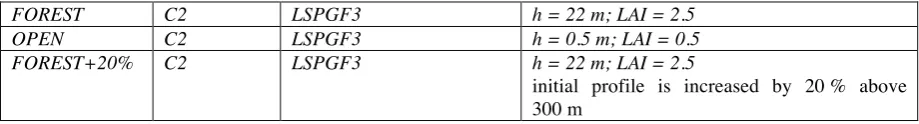
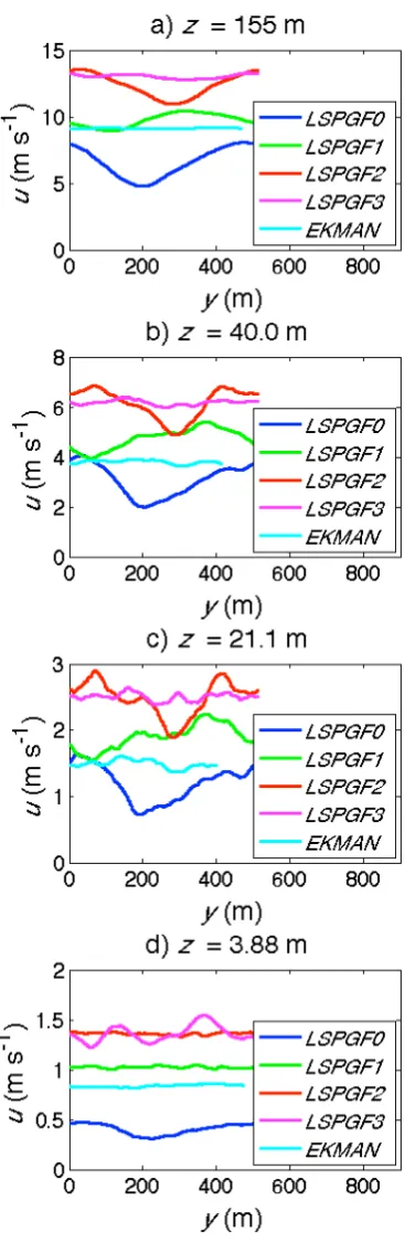
In Figure 8, the average streamwise wind velocity at heights of 155 m, 40 m, 21.1 m and 3.88
469
m between 3000 and 4000 s as a function of crosswind position (y-axis for all cases except
470
Ekman) illustrate the dependence of streak-induced streamwise velocity variations on height.
471
The peaks are associated with fast flow zones whereas the low values are associated with
472
slow flow regions. Again, LSPGF0 is characterized by the most dominant “streak pattern”
473
with a very significant difference between slow and fast regimes. LSPGF1 and LSPGF2 have
474
similar patterns at all heights even if the magnitude is not as strong. LSPGF3 shows much
475
more reasonable patterns, even if some small oscillations can be seen in the very lower part of
476
the domain.
478
Fig. 7 479
Mean wind normalized velocity at height 40 m, averaged between 3000 and 4000 s
482
Fig. 8 483
Wind velocity along the crosswise direction, averaged along the streamwise direction and
484
between 3000 and 4000 s at four different heights. For all runs except EKMAN, the crosswise
485
direction is the y-direction, whereas the streamwise is the x-direction
486 487
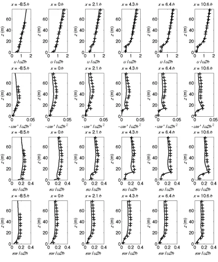
4.2 Validation of the model incorporating LSPGF against 4 experimental data
488
sets
Based on the results shown in Sect. 4.1, LSPGF3 seems to have the most desirable properties
491
(wind velocity prescription capability, reasonable streaks). Similar runs were run using
492
LSPGF3, but with the three different canopy types (C2, C3 and C4, see Table 2) in order to
493
compare simulated wind statistics against experimental data in these four scenarios. The
494
results presented in Fig. 6 show that turbulent statistics are not significantly affected by the
495
different pressure gradient techniques (with the exception of LSPGF0 for the momentum
496
flux). The validation presented here does not attempt to demonstrate that the use of LSPGF3
497
improves the predictions of wind statistics compared to other pressure gradient forcing
498
techniques, but that satisfactory results can be obtained with this approach.
499
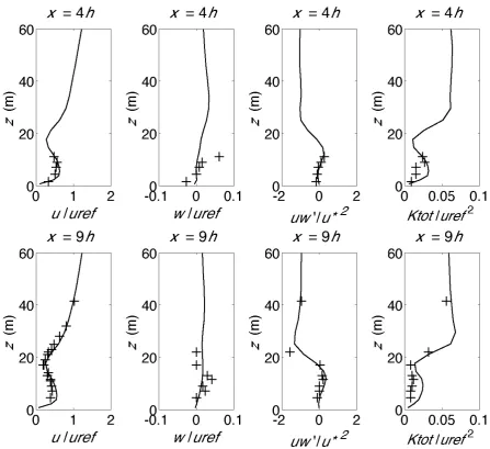
Figures 9 and 10 show the u and w velocity profiles, the momentum flux and the
500
turbulent kinetic energy profiles. These wind statistics were normalized by mean wind
501
velocity at 40 m uref for u and w velocities, by square of the friction velocity for momentum
502
flux and by uref2 for turbulent kinetic energy as in Dupont et al. (2011). Figure 9 shows those
503
profiles for the homogeneous forest (C1), whereas Fig. 10 shows them at two different
504
distances from the edge (4h and 9h) in the case of the open to forest transition (C2). The
505
model used with LSPGF3 performed well with respect to reproducing experimental data.
506
However, some discrepancies can be observed: overestimation of wind velocities below the
507
canopy in the edge case, underestimation of the momentum flux peak just above the canopy,
508
overestimation of turbulent kinetic energy below the canopy and high above it. Similar
509
differences were found in Dupont et al. (2011). It is beyond the scope of the present paper to
510
investigate the hypotheses mentioned by these authors to explain the discrepancies.
511 512 513
514
515
Fig. 9 516
Simulated wind statistics over canopy C1 with LSPGF3 (lines), against experimental data
517
(+’s)
519
520
Fig. 10 521
Simulated wind statistics over canopy C2 with LSPGF3 (lines), against experimental data
522
(+’s)
525
526
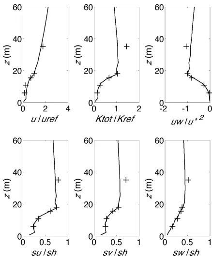
Fig. 11 527
Simulated wind statistics over canopy C3 with LSPGF3 (lines), against experimental data
528
(+’s). su, sv and sw respectively represent the standard deviation of u, v and w velocity. sh is
529
half the square root of Kref, which is turbulent kinetic energy at canopy top
530 531
For canopy C3, u velocity was normalized by uref (wind velocity at 2h = 36 m). Turbulent
532
kinetic energy was normalized by its value at canopy top (18 m). Momentum flux was
533
normalized by the square of friction velocity. Standard deviation of u, v and w were
534
normalized by the standard deviation of twice the square root of turbulent kinetic energy at
535
canopy top (18 m), as in Pimont et al. (2009). Using LSPGF3, the model provides similar
results to those of Pimont et al. (2009), who did not use any pressure gradient (Fig. 11). A
537
similar underestimation of turbulent kinetic energy at twice the height of the canopy was
538
observed, which is contrary to the overestimation seen in Fig. 9.
539 540
Canopy C4 was extrapolated from a wind tunnel experiment. The experimental data set
541
contains vertical wind statistic profiles at 6 different locations, before and after the forest
542
edge. Mean velocity, momentum flux, standard deviation of u and w velocities are available
543
and within this experimental data set all data are normalized by a single quantity u2h, which
544
is the u velocity at twice the height of the canopy at the location of the edge (except
545
momentum flux that was normalized by (u2h)2 for unit consistency). The model performance
546
with LSPGF3 was found satisfactory and of similar quality as previous studies (Dupont et al.
547
2008b; Pimont et al. 2009; Sauer 2013), with a general underestimation of turbulence
548
quantities above the canopy (Fig. 12).
550
551
Fig. 12 552
Simulated wind statistics over extrapolated canopy C4 with LSPGF3 (lines), against
553
experimental data (+’s). su and sw represent the standard deviation of u and w velocity. u2h is
554
the mean wind velocity at z = 2h and x = 0h
555 556 557
5 Discussion
558 559
5.1 Limitations of existing approaches
The scenario investigated using a geostrophic wind and the Coriolis force (simulation
562
EKMAN) illustrates the benefits and drawbacks of this approach. The benefits are a
563
convergence of the flow, reasonable wind profile and statistics, and realistic large structures
564
(streaks) due to the Ekman balance. However, the magnitude of the wind velocity in the
565
canopy neighborhood can only be controlled by the value of the geostrophic wind. Even when
566
realistic initial profiles are used (Appendix A), the convergence in the lower part of the
567
canopy can be far from the expected value (3.8 m s-1 instead of 6 m s-1), which is a major
568
drawback. This can be solved by trial and error methods, however this is expensive with
569
respect to both time and computational resources.
570 571
The wind direction is an even more serious issue. First, there is a swing that varies from 38 °
572
to 70 ° between the specified geostrophic wind and wind at various locations close to the
573
ground, so that the direction at a given height cannot be anticipated. As described above for
574
wind velocity, the requirement of managing the wind direction near the canopy by prescribing
575
the direction at the top of the domain raises a significant problem for practical use. In
576
addition, the swing between the top and bottom of the canopy was not observed in the field
577
(Dupont et al. 2011) and thus questionable. Swings have been reported in deep and dense
578
canopies (Smith et al. 1972; Shinn, 1971 cited by Wilson and Flesch 1999), but the present
579
canopy is not very dense. In Moeng and Sullivan (1994), the resolution is coarse compared to
580
vegetation and the swing induced by the Coriolis force within the surface layer is not
581
resolved. Dupont et al. (2011) reported a similar swing in their simulation, with a wind that
582
tends to align with the mesoscale pressure gradient. Below the canopy, wind velocities are so
583
small that Coriolis and drag forces become negligible compared to the pressure gradient itself
584
(Smith et al. 1972). The assumption of a constant mesoscale pressure gradient over the whole
585
domain might explain this potential overestimation of the role played by the Coriolis force in
586
the lower part of the domain. Indeed, the wind in the lower part of the domain is far from
587
being tangential to the mesoscale pressure gradient, so that the mass is transported along the
588
gradient. In the reality, over several thousands of seconds, this mass transport should reduce
589
the mesoscale pressure gradient near the ground. This is not accounted for in cyclic
590
simulations that implement the Ekman balance, assuming a constant mesoscale pressure
591
gradient everywhere. The potential overestimation of the mesoscale pressure gradient in the
592
lower part of the domain might be the reason for the swing overestimation in cyclic runs close
593
to the ground. Another point is the fact that it is unclear to the authors if these strong changes
594
in direction in the lower part of the domain are realistically accounted for in the case of
595
heterogeneous vegetation because of cyclic boundary conditions. Indeed, the wind direction at
596
a given height can be significantly different inside a forest and in a clearing for example,
597
resulting in a confusing situation. Beyond these aspects, our simulations confirm that the lack
598
of control over wind magnitude and direction close to the canopy and the potential over
599
estimation of the swing in the canopy when using Ekman balance with cyclic boundary
600
conditions is not appropriate for well-controlled stand-scale canopy wind simulations, such as
601
those required for wildland fire studies.
602 603
When no pressure gradient is used, the simulation LSPGF0 illustrates that the wind flow
604
decays with time (5 % every 200 s), before converging very slowly (about 4000 s here) to a
605
typical S profile for the u-velocity and to a constant momentum flux above the canopy, as
606
already observed by Watanabe (2004). The convergence occurs when the gradient at the top
607
is strong enough to induce sufficient flux of momentum from the damping layer into the
608
domain to balance the loss of momentum due to the vegetation drag. The present work
609
confirms the lack of control on the wind velocity at a given height and the formation of
unrealistic large streaks, reported by (Pimont et al. 2011). The limitations of the
spatially-611
constant pressure gradient have already been detailed in Sect. 1.
612 613
5.2
LSPGF
614615
The LSPGF1 presented in the present paper is an adaptation of the constant pressure gradient
616
approach, but instead of being constant, it uses a vertical profile that mimics the Ekman
617
spiral, so that the pressure gradient effects vanish at the domain top, as is the case in the
618
geostrophic layer along geostrophic wind direction. When used with realistic initial wind
619
profile and geostrophic wind, LSPGF1 is more satisfactory than LSPGF0 and EKMAN to
620
control wind velocity at a given height, because wind velocity at 40 m is closer to 5, when
621
6 m s-1 was expected. However, the control on wind magnitude is not perfect and unrealistic
622
streaks still exist, even if their magnitude is significantly lower than without pressure
623
gradient. LSPGF1 is thus an adaptation of a spatially-constant pressure gradient, that is
624
compatible with Rayleigh damping layer and planetary boundary layer modeling, but it does
625
not solve entirely the lack of control over wind magnitude close to the canopy and the
626
unrealistic streak development. A trial and error approach should be be used to refine the
627
resultant targeted wind speed.
628 629
LSPGF2 uses the integrated momentum at a given height (here 40 m) instead of the whole
630
domain as for LSPGF1. Owing to the fact that it was designed with that objective, the wind
631
velocity control in the lower part of the domain is quite satisfactory (6.1 m s-1 at 40 m with a
632
target wind of 6 m s-1). However, unrealistic streaks are still present. More generally, the
633
approaches based on a pressure gradient that is constant across horizontal planes at a given
634
height (constant pressure gradient force, LSPGF0, LSPGF1, LSPGF2) have a convergence of
635
the mean flow at each height, but there is no mechanism (except shear) to limit the
636
development of streaks of large magnitude.
637 638
LSPGF3 uses the same formulation as LSPGF2, except that the pressure gradient is
non-639
uniform in the crosswise direction in order to limit induced streak strength. This is similar to
640
EKMAN, in which the combination of Coriolis and mesoscale pressure gradient is not
641
uniform across a horizontal plane and tends to dampen streaks. Simulations show that the
642
control on wind velocity at 40 m is near-optimal and that the magnitude of the streak is very
643
limited. In addition, two fast lanes and two slow lanes are observed on the 512 m wide, which
644
is the same as the EKMAN approach, with a ratio between slow and fast regions that is similar
645
as well. LSPGF3 seems to solve most of the issues described in the introduction:
646
compatibility a Rayleigh damping layer at the domain top, control in steering towards
647
targeted wind magnitude and direction at a specific reference height in the lower part of the
648
domain, convergence of the wind profile, and realistic transient large structures (streaks). The
649
fact that the wind direction does not change with elevation under LSPGF3 is seen as
650
improving the utility of the formulation for the study of phenomena occurring in or just above
651
the canopy where the swing in the profile at higher altitudes is not of much interest. This lack
652
of swing with elevation simplifies the analysis of simple scenarios and the wind direction
653
close to the canopy is easy to control. However, the rotation induced by the Coriolis force is
654
present in the real world (even if it is generally slower than the one usually obtained in
655
EKMAN simulations) and induces a specific shear. For applications in which wind velocity
656
and direction need to be controlled but for which the rotation induced by Coriolis is likely to
657
be important, LSPGF3 could be adapted by using the Ekman spiral equations to impose a
658
controlled rotation of the mean profile. Compared to the standard EKMAN balance, the extra
rotation in the lower part of the domain would then be avoided and the wind direction at a
660
given height could be controlled.
661 662
The model with incorporation of LSPGF3 provides control over wind speed and direction and
663
generates reasonable large structure, but also performed well against the 4 experimental data
664
sets presented here. It sometimes over or underestimates some turbulent quantities, but profile
665
shapes and quantitative values are always in close agreement with experimental data, with a
666
single value of drag coefficient in all cases. Similar results were obtained with LSPGF0,
667
LSPGF1 and LSPGF2 and are not quantitatively different from the results of Su et al. (1998),
668
Yang et al. (2006), Dupont and Brunet (2008 a&b), Pimont et al. (2009), Dupont et al. (2011)
669
who used classical pressure gradient techniques (no pressure gradient, spatially-constant
670
pressure gradient, Ekman balance). The similar performance of these different techniques is
671
explained by the fact that the forcing associated with large-scale pressure gradient is very
672
weak against vegetation drag. In the case of canopy C1, Fig. 6 demonstrates that similar wind
673
statistics are obtained after normalization by wind intensity for the different pressure
674
gradients. It is especially the case in the mean wind profile where the only difference that can
675
be noticed below 80 m, is a slightly slower velocity below the canopy than obtained in the
676
case without pressure gradient. At this location, drag forces are of the same order of
677
magnitude as the pressure gradient, because velocities are very small so drag is small whereas
678
departure from geostrophic wind (Ug-u) highest. This is in agreement with findings of Dupont
679
et al. (2011), who demonstrated that the large-scale pressure gradient was responsible for the
680
secondary maximum of wind velocity below the canopy.
681 682
5.3 Sensitivity of the
LSPGF
approaches to initial profile, geostrophic wind and
683
update frequency parameter (
Δ
t
)
684 685
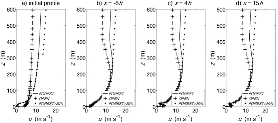
One limitation of the LSPGF approach is a potential sensitivity to initial profile (for LSPGF1)
686
and geostrophic wind (for LPGF1,2,3). LSPGF1 depends significantly on the initial profile
687
because this initial profile is used as a reference for the integrated momentum Meq in our
688
implementation. The sensitivity of LSPGF2 and LSPGF3 to initial profile and geostrophic
689
values is very limited in the lower part of the domain. This is illustrated on Fig. 13, where
690
three runs using different initial wind profiles (“FOREST”, “OPEN” and “FOREST+20%”,
691
Table 3) are compared. The case-specific initial profiles used for these three runs are shown in
692
Fig. 13a. The geostrophic wind specified at 615 m are 12.5 m s-1, 8.33 m s-1 and 15 m s-1 for
693
FOREST, OPEN and FOREST+20% respectively. Figures 13b, c and d plot the wind profiles
694
at a distance of 8h upstream of the forest edge (in the open area), 4h and 15h downstream of
695
the forest edge respectively. The modeled velocity profiles are almost identical across the
696
three cases (without normalization) below 150 m, illustrating that the sensitivity to the
697
geostrophic wind and initial condition profile is weak. However, the decline of wind velocity
698
above 200 m for the OPEN case shows that a geostrophic wind speed of 8.33 m s-1 for a
699
targeted 6 m s-1 wind speed at 40 m is inappropriate for this mix of open and tall forest.
700 701
Prescribing stronger geostrophic wind velocities can help to achieve more realistic profiles
702
aloft as illustrated by case FOREST+20%. In this case (Fig. 13b, c, and d), the profile has a
703
realistic and appropriate shape in the region above 300m. The value of 20 % velocity increase
704
was chosen because when using LSPGF1 with C1, the value of the wind velocity at 40 m was
705
20 % lower than the targeted 6 m s-1. This suggests that the integrated momentum computed
706
with profile of Appendix A was 20 % too low to achieve the targeted velocity at 40 m.
The empirical profiles described in Appendix A are satisfactory to get a first estimate of the
709
geostrophic wind required for LSPGF2 and LSPGF3. Since the sensitivity of computation in
710
the zone of interest (close to the forest, in the lowest third of the domain) is low, they can be
711
considered sufficient for most applications. For other applications such as investigation of
712
plume dynamics where flow patterns aloft are of paramount importance, more realistic
713
ambient conditions are required throughout the planetary boundary layer (i.e. the upper
two-714
thirds of the domain). In the present simulations, it seems that a geostrophic wind prescribed
715
20% higher than the value derived from the method described in the Appendix A helped to
716
achieve such a velocity profile. However when the focus shifts from the surface and canopy
717
winds to those in above the upper part of a plume, much larger horizontal domains must be
718
used and neglecting Coriolis force or assuming a constant mesoscale pressure gradient is
719
likely not satisfactory. Instead of running the model under idealized scenarios with cyclic
720
boundary conditions, it would be better to prescribed ambient variables (potential
721
temperature, pressure, wind velocities) modeled with mesoscale model such as WRF or
722
COAMPS.
723 724
725
Fig. 13 726
FOREST, OPEN and FOREST+20%: Initial parameterized wind profiles (a) and computed
727
wind profiles at 3 streamwise locations measured from the canopy edge, (b) x = -8h, (c) x =
728
4h, and (d) x = 15h. The geostrophic wind specified at 615 m were 12.5, 8.3, and 15 m s-1 for
729
FOREST, OPEN and FOREST+20%, respectively
730 731
In the LSPGF approach, a value must be given to the parameter Δt, the frequency period at
732
which an update of pressure gradient forcing is calculated. In the simulations presented here,
733
we choose Δt = 200 s as stated in Sect. 3. This value was taken because the decay rate of
734
integrated momentum using LSPGF0 in the lower part of the domain was about 5 % every
735
200 s, so that 200 s can be seen as a characteristic time of large-scale pressure gradient force
736
action on the mean flow. We also tested values 100 and 400 s and found the results to be
737
relatively insensitive within this range of parameter values. However, some high frequency
738
oscillations of the wind flow with time can appear in the lower part of the domain when Δt is
739
to small (10 s), due to the fact that the value of f is modified much faster than the time it takes
740
for the LSPGF to modify the mean flow. In contrast, when choosing Δt too large (2000 s),
741
some slow oscillations in the integrated momentum can appear. It is likely that a good choice
742
for Δt will vary when used in significantly different conditions (domain size, especially dense