Estimating Average Growth Trajectories in
Shape-Space Using Kernel Smoothing
Tim J. Hutton*, Student Member, IEEE, Bernard F. Buxton, Member, IEEE, Peter Hammond, and Henry W. W. Potts
Abstract—In this paper, we show how a dense surface point distribution model of the human face can be computed and demonstrate the usefulness of the high-dimensional shape-space for expressing the shape changes associated with growth and aging. We show how average growth trajectories for the human face can be computed in the absence of longitudinal data by using kernel smoothing across a population. A training set of three-di-mensional surface scans of 199 male and 201 female subjects of between 0 and 50 years of age is used to build the model.
Index Terms—Deformable models, facial growth, medical image registration, morphometrics.
I. INTRODUCTION
T
HERE ARE many changes in the shape of an individual’s face over time. In young adults, there is considerable growth of the skeletal structures, along with an increase in muscle tissue and changes in the volume of fatty tissues. In middle life, there is little change in the bone structure but continued growth in cartilage, especially in men, affecting amongst other things the shape of the nose. In later life, changes in both muscle tone and skin elasticity affect the outer shape of the face considerably. The modeling and prediction of these changes is a challenging task.A previous paper [1] introduced dense surface point distribu-tion models of the human face. The core of the procedure is the computation of a high-dimensional face-shape-space in which each example in the training set is represented as a point. Be-cause each vertex in a dense mesh of the face is a landmark in the model, the shape-space is of sufficiently high dimension-ality to capture subtle features of the face such as those asso-ciated with gender differences and facial dysmorphologies [2], [3]. This makes it useful for delineating between different sub-groups in a population, as was described in [1]. This high dimen-sionality of the shape-space also makes it useful for analyzing continuous parameters, such as the age of an individual, which we will study in this paper.
Manuscript received June 26, 2002; revised December 30, 2002. Asterisk
indicates corresponding author.
*T. J. Hutton is with the Biomedical Informatics Unit, Eastman Dental Institute for Oral Health Care Sciences, University College London, 256 Gray’s Inn Road, London WC1X 8LD, U.K. (e-mail: [email protected]).
B. F. Buxton is with the Department of Computer Science, University College London, London WC1E 6BT, U.K.
P. Hammond is with the Biomedical Informatics Unit, Eastman Dental Institute for Oral Health Care Sciences, University College London, London WC1X 8LD, U.K.
H. W. W. Potts is with the Cancer Research U.K. London Psychosocial Group, Guy’s, King’s, and St. Thomas’ School of Medicine, Adamson Centre for Mental Health, St. Thomas’ Hospital, London SE1 7EH, U.K.
Digital Object Identifier 10.1109/TMI.2003.814784
While some studies have analyzed three-dimensional (3-D) longitudinal data [4], [5], to date there has not been much human data available. This is partly because the development of useful acquisition technologies has only occurred recently. Another factor is that X-ray and X-ray computed tomography (CT) imaging as used in [4] and [5] have an associated radiation dosage that precludes their use on healthy individuals.
Dean et al. [4] used 3-D landmarks acquired from the Bolton standards collection of frontal and lateral head radiographs taken repeatedly for the same individuals over time. They used Procrustes methods of shape analysis to register and compare sets of landmarks across the skull of 32 individuals (16 male, 16 female) at yearly intervals between the ages of 3 and 18.
Andresen et al. [5] used CT scans of the mandible of six chil-dren (four male, two female) up to the age of 12 years. A surface model was built to compare the changing shape of the mandibles over time.
The data we use in this study is generated by noncontact sur-face scanners that use natural, infrared or laser light. The data consists of a dense polygonal surface representing the captured area, with a vertex spacing typically between 0.1 and 2 mm across the face. Although we have data from a few hundred subjects, the scanning techniques were only industrially devel-oped over the last few years. It has, therefore, not (yet) been possible to carry out longitudinal studies. Without good lon-gitudinal data, we thus consider a method that computes an aging trajectory for the average individual, from a population that spans a large age range. If the pattern of growth is not sig-nificantly different between healthy individuals of the same sex, as was found in [4], then the average aging trajectory will cap-ture the pattern of normal growth and can be used to predict the change in shape of an individual’s face as they get older. (We showed an example of this on the BBC Science program Teen Species, first screened in 2002.)
A trajectory in the space spanned by the principal components of shape variation (a shape-space) is a natural way of expressing growth. The technique is used in both [4] and [5] to show the correlation between age and the first principal component of shape variation.
In this paper, we first review the construction of the dense surface point distribution model for computing the face-shape-space and then look at the use of kernel smoothing to compute growth trajectories in this space.
II. MATERIALS ANDMETHOD
The training set consisted of 400 face scans of dif-ferent people, acquired on a DSP400 face scanner
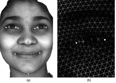
Fig. 1. An example scan with our nine landmarks (a) and a detail of the mesh around the left eye with two landmarks visible (b).
Fig. 2. The age distribution of our training set of 400 faces.
(http://www.3dmd.com). Each scan results in a triangu-lated surface mesh model of the subject’s face with between 2000 and 10 000 vertices (see Fig. 1). The nature of the acquisition is such that structures other than the face area of interest are frequently included. The model-building method deals with these automatically as we shall show.
We restricted our study to the range of 0–50 years because of a relative lack of data on people aged above 50. Fig. 2 shows the distribution of our 400 subjects across different ages. One hundred ninety-nine of the subjects were male, 201 female. The people were from all ethnic backgrounds and most scans were taken with an approximately neutral facial expression.
A. Building the Dense Surface Model
The first step is to make a dense correspondence between all the surface meshes. Methods exist for doing this automati-cally in two-dimensional (2-D) [6] and on closed surfaces in 3-D [7], but our aim here is to create a biologically accurate model and, thus, we must reduce the correspondence errors as much as possible. Our starting point is, therefore, to use hand-placed landmarks at points of high reproducibility that are biologically homologous. However, there are not many such points on the human face. The ends of the eyebrows, for example, can be ac-curately located on many faces but do not correspond biologi-cally across subjects because of the possibility of cosmetic al-teration (plucking). Other landmarks such as on the cheekbones (e.g., zygion) are biologically homologous on the hard tissue, but cannot be placed accurately on surface scans of the soft tissue because the underlying bones cannot be seen.
One other consideration for the choice of landmarks is that there be a reasonable number in the areas of the face of interest
for the purposes of creating a model with acceptable correspon-dence. For example, if we had no landmarks on the lower face, then we should not expect the correspondence in that area to be well-defined. Thus, our choice of landmarks reflects our interest in the various features of the face. For this study of facial growth, we chose the following nine landmarks: the corners of the eyes and mouth, the tip of the nose, soft-tissue nasion (bridge of the nose), and a chin point. Fig. 1 shows an example mesh with these landmarks in place.
Points in between these well-defined landmarks, such as on the cheeks and across the forehead have no precise biological correspondence and yet aspects of their shape contain useful biological information. Our method makes use of this extra information by interpolating the correspondence between the landmarks. For our interpolating function, we use the thin-plate spline (TPS) [8], which is often used for medical image analysis because it minimizes the bending energy of the transform, hence keeping distortion of the surface scans to a minimum.
The registration of the surfaces could be done using any set of landmarks as a frame of reference, but it is desirable that the landmarks are representative of the shape distribution, so we have used the generalized Procrustes algorithm [9] to compute the mean landmarks. The key step in this process is a least-squares alignment of two sets of 3-D landmarks, for which we use the quaternion method described for example in [10]. Each surface is then TPS-warped onto the mean landmarks. This registration step removes the most significant shape variation in the surfaces, as well as all of the location and orientation differences.
Having brought all the surfaces into close alignment, a dense correspondence is made by taking the closest point on each sur-face from each vertex in a base mesh. We used as a base mesh one of the examples in the training set that was particularly good regarding coverage and lack of holes. Beyond these considera-tions the choice of which example to use as a base mesh is not critical; in Section III, we will look at the effect of this (Fig. 7). The scans in the training set (including the base mesh) often included significant neck and ear areas that were not present in all the examples. We snip off these areas by using only those vertices where the maximum distance from the base mesh to the surface of each scan (after alignment) is less than 20 mm (found through experiment). While this distance is, of course, application-specific, this technique is very effective in restricting the model to those regions of the face surface that are well-represented in the training data. Essentially, we are taking an intersection of the meshes of the subject’s scans; keeping only those areas that are well-covered in all the examples.
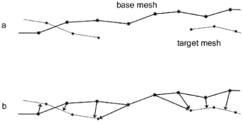
Additionally, the scans used in the training set may have small holes, misplaced vertices, or even triangulation errors, causing them not to be locally manifold. Because our method uses one mesh to sample the others by finding the closest point, it is ro-bust to such errors. For example, if there is a spike in one of the surfaces (one significantly misplaced vertex) then, since the sur-faces are in close alignment, the spike is unlikely to be sampled. This is illustrated in Fig. 3.
Similarly, a hole in a target mesh will result in the base mesh sampling points around the edge of the hole (Fig. 4).
Fig. 3. A spike (a) in the target mesh is unlikely to be sampled by the base mesh, resulting not in a large displacement vertically but a small displacement sideways.
Fig. 4. A hole in the target mesh (a) will cause the base mesh points to sample around the edges (b), again resulting in a displacement sideways.
Fig. 5. Dense correspondence algorithm illustrated. The original mesh is first TPS-warped (1) into alignment with the base mesh. The warped mesh is then resampled by finding the nearest point to each vertex of the base mesh (2). Finally, the resampled vertex is returned to the same relative position within the corresponding triangle on the original mesh (3).
with the other shape changes and are, therefore, not represented in the most significant principal components.
When the dense correspondence with a base mesh has been made, the connectivity of the base mesh can be applied to the points of correspondence in each mesh to give a set of new meshes. To return these meshes to their original shapes, we find the barycentric coordinates of the resampled vertex within the triangle on the warped mesh that contained it and move the vertex to the same relative position in the corresponding triangle in the original surface. Fig. 5 illustrates the whole process.
Now that we have constructed a dense mesh of corresponding vertices on the surface of each of the scans, we can treat all the vertices as landmarks. Following [11], we first apply the Procrustes algorithm to align all the shapes and produce a mean shape. Because our data is calibrated for size, we do not include scaling in the Procrustes alignment, but instead build a size-and-shape model [12].
A statistical model and face-shape-space is constructed by ap-plying principal components analysis to the data obtained from the above Procrustes alignment. As usual [11], each example can be represented by a shape vector of concatenated , and
coordinates for all vertices
(1)
The mean shape vector is given by
(2)
where is the number of examples in the training set. We compute the matrix using
(3)
and then, using the Eckart–Young theorem [13], we eigende-compose not the usual 3 3 covariance matrix but instead (for efficiency) the matrix
(4)
to compute the eigenvalues . The eigenvectors we are interested in are given by , where are the eigenvec-tors of . As usual, each eigenvector is then normalized to unit length.
The computed eigenvectors can be treated as deformations of the whole mesh and can be added directly to the coordinates of the vertices of the mean mesh to synthesize new faces (see for example [11])
(5)
In (5), is the matrix of the eigenvectors and is a set of parameters controlling the modes of shape variation.
The coordinates in shape-space of any example can be found using
(6)
B. Computing Average Age Trajectories Using Kernel Smoothing
The examples in the training set can now be represented as points in a shape-space. Crucially, the metric of the space is a measure of the similarity in shape and size—the partial Procrustes distance [12]. This means that intuitive operations such as interpolation and partitioning are meaningful. (If we had included scaling in the model the metric would be the full Procrustes distance.)
Kernel smoothing is a standard statistical tool for filtering out high-frequency noise from signals with a lower frequency variation. Here, we use the technique across the population of the training set to compute an average face for any given age, using weighted support from the examples that are close to the target age. The kernel serves both to interpolate between the examples (since we may have no examples at exactly the age we want) and to average out the variation due to individual subjects which we are not interested in and treat as noise.
females. We do this because it is well-known (see for example [14]) that there is a difference in the timing and types of facial growth between men and women, and we would like to see this emerge from the data.
The path of the average aging trajectory is parameterized by the target age and given by
(7)
where is the size of the population, and and are, re-spectively, the age and location in shape-space of the th subject.
We use a triangular kernel, defined by
(8)
but a Gaussian kernel was found to give very similar results. The width of the kernel is a parameter that is determined by the amount of input data and its distribution. Smaller values tend to introduce noise into the trajectory since it becomes in-fluenced by individual examples, while values that are too large will tend to smooth out the variation in which we are interested. For this dataset, we found that a years retained the difference in shape between the two groups while giving smooth curves. This seems rather large and perhaps reflects the fact that 200 faces per group over a span of 50 years is not very much data when trying to model the entire surface of the face at small time intervals. Larger populations would allow the use of smaller width values. In Fig. 13, we will look at the effect of using kernels of different widths.
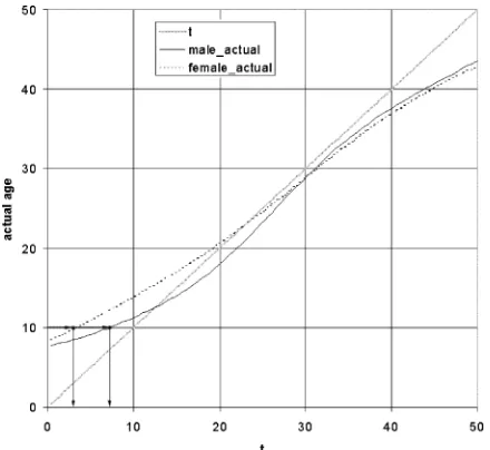
One effect of using kernel smoothing is that the width of the kernel limits how close to each end of the parameter range estimates can be made. For example, when we compute (new-born baby) we will get a weighted average that will look too old since only older faces were available in the average. This results in a face that is older than one would expect at the lower end, and a younger than expected face at the upper end of the age range. We can compute a value for a more realistic age of each average using
(9)
The plot of versus in Fig. 6 shows the typical rounding off at each end of the age range. Since is monotonically increasing with we can use this relationship to infer a unique value for a desired age. For example, to get an acceptable 10-year old average face, we need for the male subgroup and for the female subgroup. This differ-ence is caused by the varying numbers of examples at different ages for the two sexes. Table I summarizes the values used to produce Fig. 14.
III. RESULTS
A. Examining the Model
Fig. 7 shows four means computed using different base meshes picked at random, showing that the choice of base mesh does not affect the model significantly. The mottled appearance tells us that the means are very similar in shape. We
Fig. 6. A plot ofage(a(t)) versus t shows how the extremes of the age range are rounded off. At the lower end the faces are older than their correspondingt values while at the upper end they are younger. We allow for this by using the value oft needed to obtain the face of the correct age.
TABLE I
TABLE OFDESIREDAGES AND THENECESSARYVALUES OFt FOR THEMALE ANDFEMALESUBGROUPS
Fig. 7. Mean face shape computed using four different base meshes picked at random. The surfaces are rendered in different colors, the mottled appearance indicates that they are almost identical in shape.
computed the closest-point distance from each vertex on one of these surfaces to the others: 70% of the vertices are within 0.2 mm and 90% within 0.55 mm. These are comparable with the magnitude of the acquisition error and are far smaller than the shape changes captured in the most significant principal components (Fig. 8).
Fig. 8. First three modes, between03 and +3 SDs (columns), front and side views (rows).
scaling in the model in order to capture the correlation between face size and shape.
The first mode shows a strong correlation with the age of the subject (Fig. 9) while modes 2 and 3 show changes in face shape that involve identity and facial expression. Mode 3 includes fea-tures of ethnic origin difference, as well as gender. The appear-ance of these modes is essentially unchanged from the previous study [1] even though the number of examples has doubled.
For this training set of 400 examples, 43 modes are required to account for 98% of the total variation. Two previous models required 33 modes (193 examples) and 25 modes (72 examples) to account for the same 98% of the variation, showing how ex-tracting the strong correlations can give a compact representa-tion of the data. It is a typical rule of thumb (see, for example, [15]) to retain the principal components that account for 98% of the variation, as we assume the last 2% contains only noise.
A visual examination of these modes (Fig. 8) forms part of our evaluation of the efficacy of our method and the correctness of the correspondence. All of the images are plausible human faces and do not appear to have any artefacts such as ridges or distortion.
Fig. 9. First principal component plotted against the age of each person. A clear correlation is visible up to the age of 18 or so.
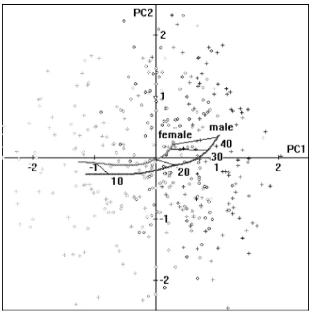
Fig. 10. Average growth trajectories for male and female, with labels marking the ages in years. The axes are the first two principal components in SDs. The scatter plot in the background shows the overall distribution of males (crosses) and females (circles).
B. Visualizing the Age Trajectory
Fig. 10 shows a plot of the two trajectories we computed against the two strongest principal components and with the corresponding ages of 10, 20, 30, and 40 marked.
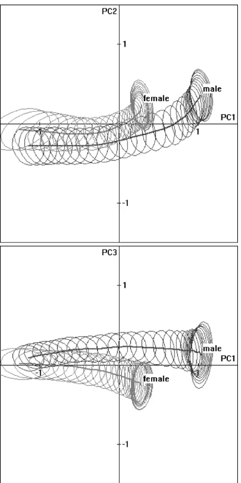
Fig. 11. Average growth trajectories for male and female, with 95% confidence regions represented as ellipses. The top plot shows the trajectories against the first two principal components, the bottom one shows the first against the third. The axes are in SDs.
the plot a confidence region of 2.45 standard deviations (SDs) is needed to include 95% of the samples. We used 10 000 boot-strap samples.
The overlap in Fig. 11 is caused by the projection into two dimensions, the trajectories are clearly separated in the full 43 dimensions of the shape-space. Fig. 12 shows the computed dis-tance between the means for all 43 dimensions plotted against age.
Fig. 13 shows the male trajectory computed using different kernel widths. Narrow kernels cause the trajectory to deviate erratically, as it becomes influenced heavily by individual ex-amples, especially where there is less data. Larger kernels give much smoother trajectories but cause the trajectory to shrink, as indicated by the end points. The effects of this shortening
Fig. 12. Euclidean distance between the means of the male and female subgroups, computed using all of the dimensions.
Fig. 13. Trajectories computed with different kernel widths of 5, 10, 15, and 20 years, shown for the male subgroup against principal components 1 and 2. For narrow kernels(width = 5) the path of the trajectory is erratic at the older end of the age range (to the right).
along the trajectory we have allowed for by using the adjust-ment method discussed earlier (Fig. 6).
Several features of these graphs are worth noting. First, the clear separation of the means (Fig. 11) demonstrates that the trajectories for males and females are significantly different. Second, a divergence of the trajectories with age can be ob-served, with the two trajectories and their confidence regions moving further away from each other as age increases. This cor-relates well with the accepted patterns of growth, where male and female face shapes become increasingly differentiated after puberty.
Third, the trajectories for the years of growth up to 18 or so are approximately linear (Figs. 10 and 11) and correlated with the first principal component (Fig. 9). This seems to match the findings of [4] and [5], even though these studies were of hard craniofacial tissues, not soft tissues. Later in life the shape-change follows a different direction, showing that over the entire lifetime the change in shape of the face is distinctly nonlinear.
Fig. 14. Synthesized faces at ages 10, 15, 20, 25, 30, 35, and 40 along the aging trajectories for females and males. The scale is the same throughout.
that the top-right face in Fig. 8 shows a distinctly masculine appearance.
Fig. 14 shows synthesized faces from along the two trajecto-ries. The seven images correspond to ages 10, 15, 20, 25, 30, 35, and 40, and were computed using the values shown in Table I.
IV. SUMMARY ANDCONCLUSION
We have described a method for creating detailed deformable models from a set of surface meshes. The method described will work on surfaces of any topology, including those with holes and unconnected regions, as long as the topology is consistent across the training set. If the topology is not consistent then the surface used to provide the base mesh will be used to sample the others and may give incorrect results. The method will work with surfaces of regular or irregular triangulation, as well as with surfaces of varying densities of triangulation.
The method is robust to occasional errors in the training data such as noisy or missing vertices. Such errors are not likely to be correlated with the other shape changes whilst the resampling according to the topology of the base mesh means they are un-likely to give rise to gross outliers. They should, therefore, only appear in the less significant modes.
We have shown how separate growth trajectories for male and female subgroups can be computed in the absence of longitu-dinal data through the use of kernel smoothing. The faces from along the two trajectories correlate well with what we think of as male and female faces of different ages. The kernel smoothing tends to roundoff the extremes of the age range, but we correct for this by using the parameter value that gives the face of the age we want.
Having a model of the pattern of normal growth is essential for studying syndromes or pathologies that cause abnormal growth. One example is Noonan Syndrome, where the growth patterns of the face change over time [17]. We would expect the average growth trajectory for individuals with Noonan Syndrome to be different to the ones shown here.
An interesting open question is to what extent the trajectory for an individual over their lifetime would be parallel to the average—this could only be answered with longitudinal data.
While we would expect the underlying patterns of growth to be broadly similar in all healthy individuals, factors such as ethnic origin, diet, and lifestyle will have an effect. Lanitis et al. [18] used sets of photos of the same individuals at different ages to build appearance models and found that the way each person’s face changes over time is different. It would be interesting to repeat this experiment using 3-D surface shape data.
ACKNOWLEDGMENT
The authors would like to thank Dr. R. Tillett of the Silsoe Research Institute for suggesting error measures on the trajec-tories. They would also like to thank the many volunteers who have allowed their scans to be used in their work. Many of the techniques used in this paper are implemented in the visual-ization toolkit (VTK) (http://www.vtk.org). The face scanner was acquired with funding from the Birth Defects Foundation (http://www.birthdefects.co.uk).
REFERENCES
[1] T. Hutton, B. Buxton, and P. Hammond, “Dense surface point distribu-tion models of the human face,” in Proc. IEEE Workshop Mathematical
Methods in Biomedical Image Analysis, Kauai, HI, 2001, pp. 153–160.
[2] P. Hammond, T. Hutton, M. Patton, and J. Allanson, “Delineation and visualization of congenital abnormality using 3D facial images,” in
Proc. Workshop Intelligent Data Analysis in Medicine and Pharma-cology (IDAMAP2001) at MedInfo2001, R. Bellazzi, B. Zupan, and X.
Liu, Eds., London, U.K., 2001, pp. 26–29.
[3] P. Hammond, T. Hutton, J. Allanson, A. Shaw, and M. Patton, “3D dig-ital stereophotogrammetric analysis of face shape in Noonan syndrome,”
J. Med. Genet., vol. 39, 2002. Suppl. 1, S35.
[4] D. Dean, M. Hans, F. Bookstein, and K. Subramanyan, “Three-dimen-sional Bolton-Brush growth study landmark data: Ontogeny and sexual dimorphism of the Bolton standards cohort,” The Cleft
Palate—Cranio-facial J., vol. 37, no. 2, pp. 145–156, 2000.
[5] P. Andresen, F. Bookstein, K. Conradsen, B. Ersbøll, J. Marsh, and S. Kreiborg, “Surface-bounded growth modeling applied to human mandibles,” IEEE Trans. Med. Imag., vol. 19, pp. 1053–1063, Nov. 2000.
[6] N. Duta, A. Jain, and M. Dubuisson-Jolly, “Automatic construction of 2D shape models,” IEEE Trans. Pattern Anal. Machine Intell., vol. 23, pp. 433–446, May 2001.
[7] R. Davies, C. Twining, T. Cootes, J. Waterton, and C. Taylor, “3D sta-tistical shape models using direct optimization of description length,” in
Proc. 7th Eur. Conf. Computer Vision, vol. 3, A. Heyden, G. Sparr, M.
Nielsen, and P. Johansen, Eds., Copenhagen, Denmark, 2002, pp. 3–20. [8] F. Bookstein, “Shape and the information in medical images: A decade of the morphometric synthesis,” Comput. Vis. Image Understand., vol. 66, no. 2, pp. 97–118, 1997.
[9] J. Gower, “Generalized procrustes analysis,” Psychometrika, vol. 40, pp. 33–51, 1975.
[10] B. Horn, “Closed-form solution of absolute orientation using unit quater-nions,” J. Opt. Soc. Amer. A, vol. 4, pp. 629–642, 1987.
[11] T. Cootes, C. Taylor, D. Cooper, and J. Graham, “Active shape models—Their training and application,” Comput. Vis. Image
Under-stand., vol. 61, no. 1, pp. 38–59, 1995.
[12] I. Dryden and K. Mardi, Statistical Shape Analysis. New York: Wiley, 1998.
[13] R. Johnson, “On the theorem stated by Eckart and Young,”
Psychome-trika, vol. 28, pp. 259–263, 1963.
[14] L. Farkas, Anthropometry of the Head and Face. New York: Raven, 1994.
[15] T. Cootes, G. Edwards, and C. Taylor, “Active appearance models,” in
Proc. Eur. Conf. Computer Vision, vol. 2, H. Burkhardt and B. Neumann,
Eds, 1998, pp. 484–498.
[16] A. Davison and D. Hinkley, Bootstrap Methods and Their Application, Cambridge, U.K.: Cambridge Univ. Press, 1997.
[17] J. Allanson, J. Hall, H. Hughes, M. Preus, and D. Witt, “Noonan syn-drome: The changing phenotype,” Amer. J. Med. Genet., vol. 21, pp. 507–514, 1985.
[18] A. Lanitis, C. Taylor, and T. Cootes, “Toward automatic simulation of aging effects on face images,” IEEE Trans. Pattern Anal. Machine