the Zero Power Analysis
Jean-Luc Danger1,2, Sylvain Guilley1,2, Philippe Hoogvorst2,
Cédric Murdica1,2, and David Naccache3
1 Secure-IC S.A.S., 80 avenue des Buttes de Coësmes, f-35700 Rennes, France
{jean-luc.danger, sylvain.guilley, cedric.murdica}@secure-ic.com 2 Département COMELEC, Institut TELECOM,
TELECOM ParisTech, CNRS LTCI, Paris, France
{jean-luc.danger, sylvain.guilley, philippe.hoogvorst, cedric.murdica}@telecom-paristech.fr 3 École normale supérieure, Département d'informatique
45, rue d'Ulm, f-75230, Paris Cedex 05, France. [email protected]
Abstract. Elliptic Curve Cryptography can be vulnerable to Side-Channel Attacks, such as the Zero Power Analysis (ZPA). This attack takes advantage of the occurrence of special points that bring a zero-value when computing a doubling or an addition of points. This paper consists in analysing this attack. Some properties of the said special points are explicited. A novel dynamic countermeasure is described. The elliptic curve formulæ are updated depending on the elliptic curve and the provided base point.
Keywords: Elliptic Curve Cryptography, Side-Channel Analysis, Zero Power Analysis, Zero-Value Points, Dynamic Countermeasure, Jacobi Symbol.
1 Introduction
Elliptic Curve Cryptography (ecc) is vulnerable to the Correlation Power Analysis [5, 3.2]. Randomizing the base point, such as the Random Projective Coordinates [5, 5.3] and the Random Curve Isomorphism [12], is an ecient way to prevent the CPA.
However, these countermeasures are not enough because of some rened attacks such as the Rened Power Analysis (RPA), introduced by Goubin [9], and its extension, the Zero Power Analysis (ZPA), introduced by Akishita and Takagi [1]. The RPA takes advantage of the occurrence or the absence of particular points of the form (0, y). These points are randomized by neither the Random Projective Coordinates nor the Random Curve Isomor-phism. The ZPA does not focus only on a zero-value in points' coordinates, but also on a possible zero-value in intermediate variables when computing a doubling or an addition of points. Such particular points are dened as zero-value points [1]. The RPA becomes a particular case of the ZPA.
The rest of the paper is structured as follows. Section 2 briey recalls on ecc and on the RPA and ZPA attacks. Section 3 is devoted to the properties of the zero-value points. Section 4 gives some existing methods to prevent the RPA and the ZPA. These methods consist in modifying the formulæ so that a zero-value point never occurs. This decreases the performance since more eld operations are required for performing doubling or addition of points. In Section 5, we expose new methods to prevent the ZPA, including:
the dynamical check that the given curve does not contain any zero-value point for doubling; the appropriate formulæ are chosen in consequence,
the modication of the base point, so that the absence of zero-value points for addition is ensured during the computation of the ecsm.
Finally, we conclude in Section 6.
2 Preliminaries
This section gives the notions on ecc and describe the attacks RPA and ZPA. This is required to fully understand the next sections.
2.1 Elliptic Curve Cryptography
An elliptic curve over a nite prime eld Fp of characteristic p >3 can be described by its
reduced Weierstraÿ form:
E:y2=x3+ax+b . (1)
with a, b ∈Fp verifying 4a3+ 27b2 6= 0. We denote by E(Fp) the set of points (x, y) ∈ F2p
satisfying equation (1), plus the point at innity O.
E(Fp) is an additive abelian group dened by the following addition law. Let P1 =
(x1, y1) 6= O and P2 = (x2, y2) 6∈ {O,−P1} be two points on E(Fp). Point addition P3 =
(x3, y3) =P1+P2 is dened by the formula:
x3 =λ2−x1−x2 y3 =λ(x1−x3)−y1
whereλ= (y
1−y2
x1−x2 if P 6=Q,
3x2 1+a
2y1 if P =Q. The inverse of point P1 is dened as−P1 = (x1,−y1).
ecc relies on the diculty of the elliptic curve discrete logarithm problem (ecdlp, computek givenP andQ= [k]P) or on the hardness of related problems such as ecdh or
ecddh, which can be solved if ecdlp can be.
2.2 Jacobian Projective Arithmetic
The equation of an elliptic curve in the Jacobian projective coordinates system in the reduced Weierstraÿ form is:
EJ:Y2=X3+aXZ4+bZ6 .
(r2X, r3Y, rZ) for all r ∈ F∗p. The point at innity is dened as O = (1,1,0) in Jacobian
coordinates.
We give addition (ecadd) and doubling (ecdbl) formulas in the Jacobian projective coordinates system. LetP1 = (X1, Y1, Z1) and P2 = (X2, Y2, Z2)two points of EJ(K).
ecdbl.P3 = (X3, Y3, Z3) = 2P1 is computed as: X3 =T, Y3 =−8Y14+M(S−T), Z3 = 2Y1Z1, where S= 4X1Y12, M = 3X12+aZ14, T =−2S+M2;
ecadd.P3 = (X3, Y3, Z3) =P1+P2 is computed as:
X3 =−H3−2U1H2+R2, Y3 =−S1H3+R(U1H2−X3), Z3 =Z1Z2H, where U1 =X1Z22, U2=X2Z12, S1=Y1Z23, S2 =Y2Z13, H =U2−U1, R=S2−S1.
ecdbl needs 4 multiplications, 6 squares and 7 additions/subtractions. ecadd needs 12 multiplications, 4 squares and 7 additions/subtractions.
Many dierent formulæ exist in the literature, such as the mixed coordinates [4] or the co-Z formulæ [13,10].
2.3 Elliptic Curve Scalar Multiplication
In ecc applications, one has to compute scalar multiplications (ecsms), i.e. compute[k]P,
givenPand an integerk. The Double-and-Add always method (Algorithm 1), secure against
the Simple Power Analysis [5], can be used to perform such a computation.
Algorithm 1 Double-and-Add always [5, 3.1] Input: k= (1, kn−2, . . . , k0)2,P
Output: [k]P R[0]←P R[1]←P
fori=n−2downto0do
R[0]←2R[0]
R[1−ki]←R[0] +P
end for returnR[0]
Applying the Double-and-Add always using ecdbl and ecadd requires16n
multiplica-tions, 10nsquares and 14nadditions/subtractions.
2.4 Rened Power Analysis
The Rened Power Analysis (RPA) introduced by Goubin [9] is based on the occurrence of the particular point P0 = (0, y) during the ecsm. The attacker chooses the base point P
such that the special point P0 will occur on certain assumptions (for example the current
targeted bit of keykis 0). The computation of such a pointP is performed as follows, with
the example of the Double-and-Add always method (Algorithm 1).
the pointP = [(kn−1, . . . , ki+1,1)2−1 mod #E]P0. The pointP0 will be doubled at iteration
i−1 only ifki= 1.
The doubling of the pointP0 can easily be detected by observing the trace, as shown in
Figure 1.
Fig. 1. Power consumption of modular multiplications of two random operands (left curve) and a random operand and zero (right curve)
2.5 Zero Power Analysis
The Zero Power Analysis (ZPA) of Akishita and Takagi [1] is an extension of the RPA. This attack does not only focus on points with a zeroxcoordinate but in intermediate values that
can possibly take the value zero when performing a doubling or an addition. Such points are called zero-value points. An elliptic curve does not necessarily contain a point of the form (0, y). In this case, the RPA cannot be applied. The ZPA brings more possible special points, and therefore can be applied to a larger set of elliptic curves.
The zero-value points depend on the formulæ used (see Section 2.2). They also depend on the way it is computed. For example, for the formula ecadd, the valueX3 can be computed
in dierent manners by changing the order of additions and subtractions. The dierent ways are analysed in [1]. In fact, we will see in Section 4 that the way X3 is computed does not
matter. A simple method permits to avoid zero-values whatever the order of additions and subtractions without any extra multiplication. We only list the conditions where a zero-value is an input of a multiplication.
On the doubling formula given in Section 2.2, the intermediate values that can take one zero-value are X1, X3 =T =−S+M2, M, S. In ane coordinates, this corresponds to the
following conditions:
x1 = 0 (D1), this corresponds toX1 = 0 and thusS = 0,
x3 = 0 (D2), this corresponds toX3 =T = 0, 3x21+a= 0(D3), this corresponds toM = 0.
Remark 1. Y1, Y3, Z1, S−T cannot be equal to zero because this would mean that the point
has order 2; Y3= 0⇒P3 has order 2; S−T = 0⇒x1 =x3 ⇒2P1=±P1 ⇒P1 has order
3 or P1 =O), which is impossible when computing the ecsm of the base point [1].
On the addition formula given in Section 2.2, the intermediate values that can take the value zero are X1, X2, X3, R. In ane coordinates, this corresponds to the following
conditions:
x1 = 0 (A1), this corresponds toX1 = 0, x2 = 0 (A2), this corresponds toX2 = 0,
x3 = 0 (A3), this corresponds toX3 = 0,
y2−y1 = 0(A4), this corresponds to R= 0.
Remark 2. Y1, Z1, Y2, Y3, Z2, H, U1H2−X3cannot be equal to zero because this would mean
that one of the points is the point at innity (Z1 = 0;Z2= 0) or one of the points has order
2 (Y1 = 0; Y2 = 0; Y3 = 0) or P1 =±P2 (H = 0⇒ x1 =x2 ⇒ P1 = ±P2) or P3 =±P1
(U1H2−X3 = 0⇒ x1 = x3), which is impossible when computing the ecsm of the base
point [1].
Remark 3. The conditions where thex coordinate is zero corresponds to the RPA attack.
For both addition and doubling, the mixed coordinates [4] and the co-Z formulæ [13,10]
bring the same conditions. This is because the numerator of λ of the formulæ in ane
coordinates is always computed.
2.6 Finding zero-value points
We give some methods for nding zero-value points to perform the ZPA, given an ellip-tic curve. Let us take for example the Double-and-Add always algorithm (Algorithm 1). Of course, the method can be adapted to other ecsms. Suppose that the attacker already knows the n−i−1leftmost bits of the xed scalar k= (kn−1, . . . , k0)2 and tries to recover ki. The attacker has several possibilities, listed hereafter.
Taking advantage of condition (D1). If the given elliptic curve contains a point of the form P0 = (0, y), the attacker can compute the point P = [(kn−1, . . . , ki+1,1)−21 mod
#E]P0. The point P0 will be doubled only if ki = 1. Taking advantage of conditions (D2),
(A1), (A2) or (A3) is similar.
Taking advantage of condition (D3). If the given elliptic curve contains a point P1 =
(x, y) such that3x2+a= 0the attacker can compute the point P = [(k
n−1, . . . , ki+1,1)−21
mod #E]P1. The point P1 will be doubled only ifki = 1.
Taking advantage of condition (A4). It is a bit more tricky. Indeed, the attacker has to nd a base point P = (xP, yP) such that Q= (xQ, yQ) = [(kn−1, . . . , ki+1,1)2]P and P
satisfy yQ−yP = 0. The best known method to nd such a pointP is to use the division
polynomials [16, 3.2]. For a positive integer m, if [m]P 6=O,[m]P can be expressed as
[m]P =
φm(x)
ψm(x)2
, ωm(x, y) ψm(x, y)3
where ψm denotes the mth division polynomial, and is recursively computed4. φm and ωm
are dened as
φm=xψ2m−ψm+1ψm−1 , ωm=
ψm+2ψm2−1−ψm−2ψ2m+1
4y .
Denote m = (kn−1, . . . , ki+1,1)2. Finding a pointP = (xP, yP) such that Q= (xQ, yQ) =
[m]P and P satisfy yQ −yP = 0, can be done as follows. First, nd xP a solution of the
following equation.
f(x, y) =ωm(x, y)−yψm(x, y)3 = 0 . (2)
Using the recursive properties of the division polynomials, and by replacingy2byx3+ax+b, f ∈Z[x]if mis even, and fy ∈Z[x]if mis odd [16, 3.2]. If x3P +axP +bis a square in Fp,
thenyP = q
x3P +axP +b.
Solving Equation 2 for largemis hard. Indeed, it consists in nding roots of polynomials
of degree m2+m which is dicult [1].
However, it is still feasible for smallm. In addition, there is no guarantee that there is no
other more ecient method to compute such a point. The protection against ZPA presented in this paper is ensured.
2.7 Isogeny defence
To protect against the RPA, Smart introduced the isogeny defence [14]. It consists in com-puting the ecsm on an isogenous curveE0that does not contain any point of the form(0, y),
instead of the given elliptic curveE. Akishita and Takagi extended later the countermeasure
to also prevent the ZPA [2].
Isogenous curves of standardized curves are precomputed and stored in the chip. Indeed, nding isogenies is not trivial and cannot be done on the y with a new given elliptic curve. The countermeasure proposed in this paper is dynamic and works on any curve.
2.8 Scalar Randomization
Randomizing the scalar, such as the group scalar randomization [5, 5.1], the additive split-ting [6, 4.2], the Euclidean splitsplit-ting [3, 4] or the multiplicative splitsplit-ting [15] are believed to be secure against the RPA and ZPA.
However, as opposed to the isogeny defence and our proposed methods, the absence of special points is not ensured with scalar randomization techniques. Since several bits can be targeted at a time with the RPA and the ZPA, the attacker can recover several bits of the randomized scalar. The system is not fully broken, nevertheless the security is compromised.
3 Properties of the Zero-Value Points
In this section, we give some properties of the zero-value points, namely, points satisfying (D1), (D3) and (A4). Given the elliptic curve E:y2 =x3+ax+b, dened over Fp, we will
see how to verify whether the curve does contain zero-value points or how to tell if a given point satises condition (A4).
3.1 P = (0, yP) (D1)
We dene the particular points with a zerox coordinate.
Denition 1. A point P ∈E of the form P = (0, yP) is called a zero x-coordinate point.
Proposition 1. E contains zerox-coordinate points over Fp i b is a square. In this case,
the zero x-coordinate points are (0,√b) and (0,−√b).
Proof. ( =⇒ ) Suppose E contains a zero x-coordinate point P = (0, yP), then (0, yP)
satises the curve equation and y2P = b =⇒ b is a square. (⇐=) If b = yP2 for some yP ∈ Fp, then the pair (0, yP) ∈ F2p satises the curve equation and therefore lies on the
curve E. In this case,(0,−yP) also lies on the curve. ut
3.2 P = (xP, yP) satisfying 3x2P +a = 0 (D3)
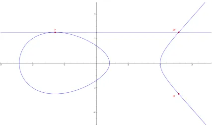
Denition 2. A point P = (xP, yP) ∈E satisfying 3x2P +a = 0 is called a zero tangent line slope point.
Fig. 2. A zero tangent line slope point on the curvey2=x3−5x+ 1overR
Proposition 2. E contains zero tangent line slope points over Fp i the two following
conditions are satised
Proof. ( =⇒) Suppose E contains a zero tangent line slope point P = (xP, yP). Then, xP
veries 3x2P +a= 0 =⇒ −a/3 is a square, and therefore −9a3 =−3a is a square because
9 is. xP can take two values:
xP =p−a/3 =δ, in this case, yP2 =xP3 +axP +b=−a3δ+aδ+b is a square, or
xP =−
p
−a/3 =−δ, in this case,yP2 =x3P +axP +b= a3δ−aδ+bis a square.
(⇐=)Suppose−3ais a square and denoteδ=p−a/3. If−a
3δ+aδ+bis a square, then the
pair (xP, yP), with xP =δ, yP =
p
−a
3δ+aδ+b, satises the curve equation and therefore
(xP, yP) lies on the curve. Moreover xP satises 3x2P +a = 0. If a3δ −aδ+b is a square,
then the pair (xP, yP), with xP =−δ, yP =
pa
3δ−aδ+bsatises the curve equation and
therefore (xP, yP) lies on the curve. MoreoverxP satises3x2P +a= 0. ut
From the proposition, we can give the following trivial corollary.
Corollary 1. If −3ais not a square, E does not contain any zero tangent line slope point.
3.3 P = (xP, yP), Q= (xQ, yQ) satisfying yP −yQ = 0 (A4)
Denition 3. A point P = (xP, yP)∈E such that there exists a point Q= (xQ, yQ)∈E,
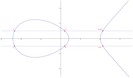
with Q6=P and yP =yQ is called a y same coordinate point.
Fig. 3. Someysame coordinate points on the curvey2=x3−5x+ 1over R
Proposition 3. Let P = (xP, yP) a point ofE with order dierent from 3. P is ay same
Proof. Let P = (xP, yP) ∈ E. By Bézout's theorem, the line y = yP has one or three
intersections, counting with multiplicity, with the curve E. Finding the intersections can
be done by solving the equation yP2 = x3+ax+b.xP is a solution, thus the equation is
equivalent to (by dividing by x−xP):
x2+xPx+x2P +a= 0 . (3)
This equation has two roots, counting with multiplicity, i the discriminant−3x2P −4ais a
square. Moreover, at least one of the root is dierent toxP, otherwise this would mean that P is the intersection of the liney=yP and E with multiplicity 3. By the addition law, this
would mean thatP+P =−P ⇒[3]P =O which is impossible by the hypothesis ofP. ut
With this proposition, the following corollary denes a set of elliptic curves that do not contain any y same coordinate point.
Corollary 2. If a= 0 and −3 is not a square in Fp, then E does not contain any y same
values point of order dierent from 3.
Proof. Suppose that a= 0 and−3is not a square in Fp, andP = (xP, yP)∈E is a ysame
coordinate point, thus −3x2P is a square and therefore −3 is square. By contradiction, E
does not contain any y same coordinate point. ut
Remark 4. On the other hand, ifa= 0 and−3is a square, all points arey same coordinate
points.
4 Modifying Formulæ
Some countermeasures consist in modifying the formulæ so that a zero value is never ma-nipulated. This prevent against the RPA and ZPA.
Itoh et al. introduced the Random Linear Coordinates [11]. It consists in replacing the pointP = (X, Y, Z)by(X0, Y, Z, µ)withµa random element inFpandX0 =X+µ, to avoid
direct manipulation ofX. The modied formulæ are protected against zerox-coordinate and
zero tangent line slope points (they omit the y same coordinate points).
Danger et al. proposed an alternative solution to prevent against zerox-coordinate points
[7]. It consists in modifying the given elliptic curve using an isomorphism to transform the base pointP = (x, y)intoP0 = (0, y0). The given elliptic curveEis mapped to a curveE0 of
the formy2 =x3+a2x2+a4x+a6.E0is not in the Weierstraÿform. Therefore, an adaptation
of the formulæ has to be done. The impact of the countermeasure is reduced because the addition withP0is simplied due to the zero value. When using co-Z formulæ, this does not
bring any additional cost. We adapted the method to the formulæ of Section 2.2 (ecdbl and ecadd), mixed with the methods described below. It turns out it is more ecient than the Random Linear Coordinates for protecting against zero x-coordinate and zero tangent
line slope points 5, only on the case where the base point, or its opposite (−P0 = (0,−y))
is frequently manipulated during the ecsm, like the Double-and-Add always method (Algo-rithm 1) and the Montgomery Ladder using co-Z formulæ [10, Algorithm 7].
We give some very trivial methods to modify the formulæ so that a zero-value can never occur. In the following,r denotes a random element ofFp.
Protecting an additions' sequence (method 1). Denotev←Pm
i=0(−1)µiuia sequence
of additions and subtractions, withm >0, µi∈ {0,1}, ui∈Fp. In order to prevent from
pos-sible zero-values that can occur during the sequence, one can simply perform the following additions' sequencet←r+Pm
i=0(−1)µiui instead, and start the sequence with the addition
of r. Then, compute u=t−r to recover the correct value u. The cost of the protection is
2 additions6.
Protecting a square (method 2). A method to protect a square u2, with u possibly
equals zero, is to compute (u+r)(u−r) =u2−r2. The correct valueu2 can be recovered
by subtracting r2. Ifr2 is precomputed, the cost of the protection is 3 additions6.
Protecting a multiplication (method 3). A method to protect a multiplicationuv, with u possibly equals zero, andv 6= 0, is to compute s= (u+r)v =uv+rv and t =rv. The
true valueuv can be recover later by computings−t. In this case, the cost of the protection
is 1 multiplication and 2 additions6.
We give addition (ecadd-d1) and doubling (ecdbl-d1-d3)7 formulas in the Jacobian
projective coordinates system. Let P1 = (X1, Y1, Z1) and P2 = (X2, Y2, Z2) two points of
E:y2=x3+a2x2+a4x+a6. We recall that, when using the method described in [7], the
addition of points is always performed with a zero x coordinate.
Algorithm 2 ecdbl-d1-d3 Input: P = (X1, Y1, Z1)∈EJ, r, s=r2 Output: 2P
S←4X1Y12; M
0←
r+ 3X2
1+ 2a2X1Z12+a4Z14
M00←M0−2r; Z3←2Y1Z1
T0←r+M0M00−2S−a2Z32−s
X3←T0−r
Y30←r−8Y14+M0(S−X3)−r(S−X3)
Y3←Y3−r return(X3, Y3, Z3)
6 By convention, and for a better clarity, we set 1 addition = 1 subtraction in terms of computational cost 7 d1-d3 means that it is protected against zerox-coordinate (condition D1) and zero tangent line slope
Algorithm 3 ecadd-d1
Input: P = (0, Y1, Z1), Q= (X2, Y2, Z2)∈EJ,
r, s=r2
Output: P+Q H ←X2Z12
S1←Y1Z23; S2←Y2Z13
R←S2−S1; Z3←Z1Z2H
X30 ←r−H3+R2−a2Z32
X3←X30−r; Y3← −S1H3−X3R return(X3, Y3, Z3)
ecdbl-d1-d3 needs 5 extra multiplications and 11 additions compared to ecdbl. ecadd-d1 needs 1 extra square and 3 additions, and 1 multiplication less compared to ecadd.
The formula below brings addition of points without any zero intermediate value.
Algorithm 4 ecadd-d1-a4
Input: P = (0, Y1, Z1), Q= (X2, Y2, Z2)∈EJ,
r, s=r2
Output: P+Q H ←X2Z12
S1←Y1Z23; S2←Y2Z13
R0←r+S2−S1; Z3←Z1Z2H
R00←R0−2r X30 ←r−H3+R
0
R00−a2Z32−s
Y30←r−S1H3−X3R0−rX3
X3←X30−r; Y3←Y30−r return(X3, Y3, Z3)
ecadd-d1-a4 needs 2 extra multiplications and 10 additions compared to ecadd.
For the Double-and-Add always (Algorithm 1), the extra cost of applying ecdbl-d1-d3 and ecadd-d1-a4 is 7n multiplications and21n additions.
5 Dynamically check the curve and the base point
Modifying the formulæ, as described in the previous section, is expensive. Sometimes, the protection is not necessary because the elliptic curve does not contain any zero-value points. In this case, the protection brings extra unnecessary computation.
We give in this section our new method to save the extra costly eld operations required for ecdbl-d1-d3 and ecadd-d1-a4 compared to ecdbl and ecadd. The given curve and the given point can be checked to remove some unnecessary protection.
of an addition/subtraction to the cost of a multiplication. It is connected to the bit length of the manipulated integers and depends on the architecture. We can refer to the analysis made by Giraud and Verneuil in [8], which is given in Table 1.
Bit length 160 192 224 256 320 384 512 521
α 0.36 0.30 0.25 0.22 0.16 0.13 0.09 0.09
Table 1. Ratio of a cost of an addition/subtraction to the cost of a multiplication given in [8]
5.1 Legendre symbol
For our new protection, we need the denition and some properties of the Legendre symbol
a p
.
Denition 4. Let p be an odd prime, and aan integer.
a p
=
1 if ais a square modulo p and a6≡0 mod p,
−1 if ais a quadratic non-residue modulo p,
0 if a≡0 mod p .
The Legendre symbol can be computed using the generalized Jacobi symbol. The fol-lowing algorithm permits to compute the Jacobi symbol.
Algorithm 5 Binary algorithm for the Jacobi symbol Input: an odd integer0< b <2n, and0< a < b, withgcd(a, b) = 1
Output: a b
J←1
α←n .bit length ofa
β←n .bit length ofb
whilea6= 1 do
whileais even do a←a/2; α←α−1
if (b= 3 mod 8orb= 5 mod 8) thenJ=−J
end while if α≤βthen
swap(a, b); swap(α, β)
if (a= 3 mod 4andb= 3 mod 4) thenJ=−J
end if
if ((a+b) = 0 mod 4) thena←(a+b)/4; α←α−1
elsea←(a+ 3b)/4
end while returnJ
The complexity of the algorithm isO(n2). However, we performed statistical tests that
reveal that the average number of additions for random values ofaand random primesb is
5.2 Checking that the curve does not contain any zero x-coordinate
Given the elliptic curve E:y2=x3+ax+b, and from Proposition 1, we can state that
if b p
= 1, then the curve might contain some zero x coordinate points,
if b p
=−1, the curve does not contain any zerox coordinate point.
One can compute the Jacobi symbol of b at the beginning of the ecsm. If
b p
= 1, then the protection against (D1) is applied. If b
p
= −1, the protection against (D1) is not necessary. In this case, we can remove the protection and save 4 multiplications and 3 additions over ecdbl-d1-d3 and 1 multiplication and 3 additions over ecadd-d1-a4.
On random elliptic curves, the probability ofbbeing a square is 1/2. The Jacobi symbol
costs1.5nadditions in average. On the Double-and-Add always method (Algorithm 1), the
performance gain is 5/2n+ 6/2αn−1.5αn= (2.5 + 1.5α)nmultiplications.
5.3 Checking that the curve does not contain any zero tangent line slope points
This case is analogous to the previous subsection. Given the elliptic curveE:y2 =x3+ax+b,
and from corollary 1, we can state that
if −3a p
= 1, then the curve might contain some zero tangent line slope points, if −3a
p
=−1, the curve does not contain any zero tangent line slope point.
One can compute the Jacobi symbol of−3aat the beginning of the ecsm. If
−3a p
= 1, then the protection against (D3) is applied. If −3a
p
=−1, the protection against (D3) is not necessary. In this case, we can remove the protection and save 1 multiplication and 8 additions over ecdbl-d1-d3.
On random elliptic curves, the probability of −3a being a square is 1/2. The Jacobi
symbol costs1.5nadditions in average. On the Double-and-Add always method (Algorithm
1), the performance gain is 1/2n+ 8/2αn−1.5αn= (0.5 + 2.5α)nmultiplications.
5.4 Checking that the base point is not a y same coordinate point
We are interested here on ecsms where the base point (or its inverse) is involved at each iteration of the ecsm, like the Double-and-Add method and the Montgomery Ladder using co-Z formulæ [10, Algorithm 7].
Given the elliptic curve E:y2 = x3 +ax+b, the base point P = (xP, yP) and from Proposition 3, we can state that
if −3x2
P−4a p
if −3x2
P−4a p
=−1,P is not a y same coordinate point.
One can compute the Jacobi symbol of −3x2P −4a at the beginning of the ecsm. If
−3x2
P−4a p
= 1, then the protection against (A4) is applied. If−3x2P−4a p
=−1, the pro-tection against (A4) is not necessary when adding the base point. We can therefore remove the protection and save 1 multiplication and 7 additions over ecadd-d1-a4.
On random elliptic curves, the probability of the base point being a y same coordinate
is 1/2. The Jacobi symbol costs 1.5n additions in average. On the Double-and-Add always
method (Algorithm 1), the performance gain is 1/2n+ 7/2αn−1.5αn= (0.5 + 2α)n
mul-tiplications.
A more ecient method to prevent from y same coordinate points is described in the
next subsection.
5.5 Modifying the base point
We propose another method to protect against (A4).
Given the elliptic curveE:y2 =x3+ax+band the base pointP = (xP, yP), the Jacobi
symbol of −3x2P−4a p
is computed to check if P is a y same coordinate point. If it is not,
the protection is not applied. If P is a y same coordinate point, rather than applying the
protection, we propose the following method illustrated in Algorithm 6.
Algorithm 6 Protected ecsm against (A4) Input: P = (xP, yP)∈E and an integerk
Output: [k]P
j←0
S= (xS, yS)←P
while−3x2
S−4a
p
= 1do
S←2S j←j+ 1
end while ComputeQ←
bk/2jc
S without protection against (A4)
ComputeR←Q+ [k mod 2j]P with protection against (A4)
returnR
After the while loop, S is not a y same coordinate point. Therefore, the protection
against (A4) is not necessary when computing Q.
After performing a point doubling, the pointSis in ane coordinates. IfS = (XS, YS, ZS)
is in Jacobian coordinates, it is equivalent to check −3X2
S−4aZ4S p
. Indeed,−3XS2−4aZS4 = (−3x2S−4a)ZS4 andZS4 is a square. With the Legendre properties,−3XS2−4aZS4 is a square
We performed a statistical study on standardized curves. Running the algorithm with random inputs,jis equal to 1 in average8. The pointRis computed under protection against
(A4), with a very small scalar (a very few bits). The computation is negligible compared to the complete ecsm. The Jacobi symbol costs 1.5nadditions in average, which is computed
2 times in average. On the Double-and-Add always method (Algorithm 1), the performance gain is n+ 7αn−3αn = (1 + 4α)n multiplications which is better than the gain of the
protection against (A4) of Section 5.4: (0.5 + 2α)nmultiplications.
6 Conclusion
An analysis on the ZPA is given. We suggest a method to dynamically check the curve and the base point. Depending on the given curve and base point, the formulæ used to perform the ecsm are dynamically adapted for protection against zero value points. The unnecessary protections are removed for eciency.
The countermeasure needs the computation of the Jacobi symbol. The performance gain of the proposed method is given with a basic software Jacobi symbol module. A dedicated embedded Jacobi symbol calculator can improve the countermeasure.
References
1. T. Akishita and T. Takagi, Zero-Value Point Attacks on Elliptic Curve Cryptosystem. Proceedings of isc'03, lncs vol. 2851, Springer-Verlag, 2003, pp. 218-233.
2. T. Akishita and T. Takagi, On the Optimal Parameter Choice for Elliptic Curve Cryptosystems Using Isogeny. Proceedings of pkc'04, lncs vol. 2947, Springer-Verlag, 2004, pp. 346-359.
3. M. Ciet and M. Joye, (Virtually) Free Randomization Techniques for Elliptic Curve Cryptography. Proceedings of icis'03, lncs vol. 2836, Springer-Verlag, 2003, pp. 348-359.
4. H. Cohen, A. Miyaji and T. Ono, Ecient Elliptic Curve Exponentiation Using Mixed Coordinates. Proceedings of asiacrypt'98, lncs vol. 1514, Springer-Verlag, 1998, pp. 51-65.
5. J.-S. Coron, Resistance against Dierential Power Analysis for Elliptic Curve Cryptosystems. Proceedings of ches'99, lncs vol. 1717, Springer-Verlag, 1999, pp. 292-302.
6. C. Clavier and M. Joye, Universal Exponentiation Algorithm. Proceedings of ches'01, lncs vol. 2162, Springer-Verlag, 2001, pp. 300-308.
7. J.-L. Danger, S. Guilley, P. Hoogvorst, C. Murdica and D. Naccache, Low-Cost Countermeasure against RPA. Proceedings of cardis'12, lncs vol. 7771, Springer-Verlag, 2013, pp. 106-122.
8. C. Giraud and V. Verneuil, Atomicity Improvement for Elliptic Curve Scalar Multiplication. Proceedings of cardis'10, lncs vol. 6035, Springer-Verlag, 2010, pp. 80-101.
9. L. Goubin, A Rened Power-Analysis Attack on Elliptic Curve Cryptosystems. Proceedings of pkc'03, lncs vol. 2567, Springer-Verlag, 2002, pp. 199-210.
10. R. R. Goundar, M. Joye and A. Miyaji, Co-Z Addition Formulæ and Binary Ladders on Elliptic Curves - (Extended Abstract). Proceedings of ches'10, lncs vol. 6225, Springer-Verlag, 2010, pp. 65-79. 11. K. Itoh, T. Izu and M. Takenaka, Ecient Countermeasures against Power Analysis for Elliptic Curve
Cryptosystems. cardis'04, Klumer, 2004, pp. 99-114.
12. M. Joye and C. Tymen, Protections against Dierential Analysis for Elliptic Curve Cryptography. Proceedings of ches'01, lncs vol. 2162, Springer-Verlag, 2001, pp. 377-390.
13. N. Meloni, New Point Addition Formulae for ecc Applications. Proceedings of waifi'07, lncs vol. 4547, Springer-Verlag, 2007, pp. 189-201.
14. N. Smart, An Analysis of Goubin's Rened Power Analysis Attack. Proceedings of ches'03, lncs vol. 2779, Springer-Verlag, 2003, pp. 281-290.
15. E. Trichina and A. Bellezza, Implementation of Elliptic Curve Cryptography with Built-In Counter Measures against Side Channel Attacks. Proceedings of ches'02, lncs vol. 2523, Springer-Verlag, 2002, pp. 98-113.
16. L. Washington Elliptic Curves: Number Theory and Cryptography, Second Edition. Chapman & Hall/CRC, 2008.
A Division Polynomials
LetE:y2 =x3+ax+bdened overFp. The division polynomialsψm ∈Fp[x, y]are dened
as:
ψ0= 0 ψ1= 1
ψ2= 2y
ψ3= 3x4+ 6ax2+ 12bx−a2
ψ4= 4y(x6+ 5ax4+ 20bx3−5a2x2−4abx−8b2−a3 ψ2m+1=ψm+2ψm3 −ψm−1ψ3m+1 for m≥2