Point Cloud Data Retrieval from 3D Geospatial
Database for Automated Road Median Extraction
Pankaj Kumar1,†*, Paul Lewis2and Conor P. McElhinney3,
1 Geomatics Division, Centre Tecnològic de Telecomunicacions de Catalunya (CTTC/CERCA), Castelldefels,
Barcelona, Spain; [email protected]
2 National Centre for Geocomputation (NCG), Maynooth University, Co. Kildare, Ireland; [email protected]
2 Amazon Web Services (AWS), Dublin, Ireland; [email protected]
* Correspondence: [email protected]; Tel.: +34-936-452-900
† Current address: Geomatics Division, Centre Tecnològic de Telecomunicacions de Catalunya (CTTC/CERCA), Castelldefels, Barcelona, Spain
Abstract: Laser scanning systems make use of Light Detection and Ranging (LiDAR) technology 1
to acquire accurately georeferenced sets of dense 3D point cloud data. The information acquired 2
using these systems produces better knowledge about the terrain objects which are inherently 3D 3
in nature. The LiDAR data acquired from mobile, airborne or terrestrial platforms provides several 4
benefit over conventional sources of data acquisition in terms of accuracy, resolution and attributes. 5
However, the large volume and scale of LiDAR data have inhibited the development of automated 6
feature extraction algorithms due to the extensive computational cost involved in it. Moreover, the 7
heterogeneously distributed point cloud, which represents objects with varying size, point density, 8
holes and complicated structures pose a great challenge for data processing. Currently, geospatial 9
database systems do not provide a robust solution for efficient storage and accessibility of raw data 10
in a way that data processing could be applied based on optimal spatial extent. In this paper, we 11
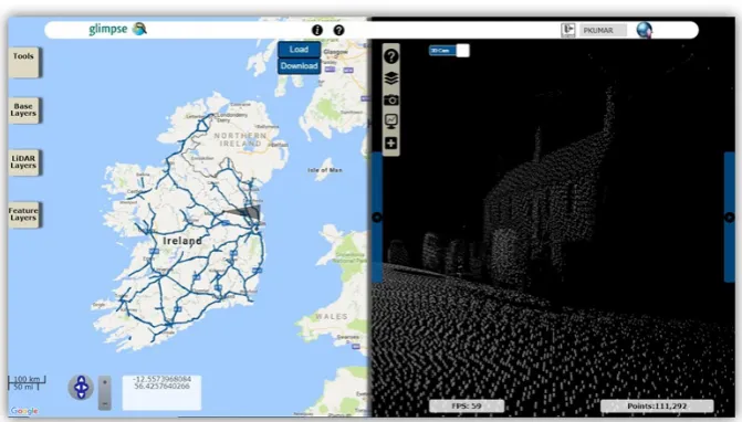
present Global LiDAR and Imagery Mobile Processing Spatial Environment (GLIMPSE) system 12
that provides a framework for storage, management and integration of 3D LiDAR data acquired 13
from multiple platforms. The system facilitates an efficient accessibility to the raw dataset, which is 14
hierarchically represented in a geographically meaningful way. We utilise the GLIMPSE system to 15
automatically extract road median from Airborne Laser Scanning (ALS) point cloud. In the first part 16
of this paper, we detail an approach to efficiently retrieve the point cloud data from the GLIMPSE 17
system for a particular geographic area based on user requirements. In the second part, we present an 18
algorithm to automatically extract road median from the retrieved LiDAR data. The developed road 19
median extraction algorithm utilises the LiDAR elevation and intensity attributes to distinguish the 20
median from the road surface. We successfully tested our algorithms on two road sections consisting 21
of distinct road median types based on concrete and grass-hedge barriers. The use of GLIMPSE 22
improved the efficiency of the road median extraction in terms of fast accessibility to ALS point cloud 23
data for the required road sections. The developed system and its associated algorithms provide a 24
comprehensive solution to the user’s requirement for an efficient storage, integration, retrieval and 25
processing of large volumes of LiDAR point cloud data. These findings and knowledge contribute to 26
a more rapid, cost-effective and comprehensive approach to surveying road networks. 27
Keywords:Airborne Laser Scanning; Geospatial Database; Data Retrieval; Road Median; Attributes 28
1. Introduction 29
Accurate 3D information about the location of real-world objects along with their geometrical and 30
structural properties supports a wide range of services and evidence based decision making. Light 31
Detection And Ranging (LiDAR) enables 3D surveying of real world environments by measuring 32
the time of return of emitted light pulses. The applicability of laser scanning systems, which use 33
LiDAR technology, continues to prove their worth due to the rapid, continuous and cost effective 34
3D data collection capability. The information obtained through these systems contributes to the 35
production of useful knowledge which can be used to develop more efficient approaches for managing 36
urban infrastructures and natural resources [1]. Their 3D data acquisition capability produces better 37
knowledge about terrain objects which are inherently 3D in nature. Laser scanning systems facilitate 38
the acquisition of an accurate, precise and georeferenced set of dense LiDAR point cloud data. Other 39
benefit of these systems is the high level of automation involved in data acquisition process and their 40
ability to acquire data beneath tree’s canopy [2]. 41
The 3D data acquired from Mobile Laser Scanning (MLS) and Airborne Laser Scanning (ALS) 42
systems differ in terms of intrinsic accuracy, resolution and object scale. This difference is incurred 43
primarily due to the distance of the scanner to the target objects, scan direction and view angle [3]. 44
Laser scanning system can facilitate reliable and accurate acquisition of 3D spatially referenced data 45
about road median, which is a narrow strip of land that separates traffic on opposite sides of the road. 46
The road median is one of the fundamental feature, whose correct identification is a prerequisite to 47
obtain precise information about road and other physical objects along it. The acquired 3D LiDAR data 48
can be used to locate, measure and classify the road median in a timely cost-effective manner in order 49
to facilitate their maintenance. This information can assist road authorities in effective management of 50
road networks and to ensure maximum safety conditions for road users [4]. 51
LiDAR data records a number of attributes including elevation, intensity, pulse width, range and 52
multiple echo information, all of which can be used for precise extraction of road median. It is a rich 53
source of 3D georeferenced information, whose volume and scale have inhibited the development of 54
automated algorithms [5]. The large volume of data produced by modern-day laser scanning systems 55
lead to time-consuming and computational expensive processes for automated features extraction. For 56
example, Riegl VQ-250 MLS generates 300,000 points per second resulting in approximately 20GB of 57
data per hour. Significant challenges exist when dealing with these volumes of LiDAR data, from its 58
storage through all stages to features extraction. The raw LiDAR data files usually contain long strips 59
of points which prohibit efficient data processing in terms of memory allocation and algorithm design 60
[6]. The acquired point cloud is heterogeneously distributed representing objects with varying size, 61
point density, holes and complicated structures, which poses a great challenge for data processing [7]. 62
While an efficient storage system for very-large 3D point cloud data is one of the key aspects for 63
information extraction. Equally important should be the ability of such a system to segment and merge 64
point clouds that are spatially coincident. However, the industrial standard has been to cluster LiDAR 65
data into spatial grids, which are then stored as binary files in a survey-based file structure. This 66
survey-based approach, that prevails in most software suites, has proven to be a major constraint in a 67
meaningful analysis of the LiDAR data [8,9]. These software suites do not provide efficient access to 68
the raw data at different or irregular spatial dimensions. It becomes challenging to access LiDAR data 69
for a particular geographical area across numerous surveys that invariably accumulate as a massive 70
dataset. The efficiency of automated processing algorithm depends upon the raw LiDAR data being 71
spatially optimised for the algorithm. The data storage system should facilitate an efficient accessibility 72
to the raw datasets in a way that data processing could be applied based on optimal spatial extent 73
and point density/resolution. This will improve the efficiency of automated algorithms in terms of 74
computation and reduced processing of the dataset. 75
In this paper, we present aGlobalLiDAR andImageryMobileProcessingSpatialEnvironment 76
(GLIMPSE) system, that provides a framework for storage, management and integration of LiDAR 77
data acquired from terrestrial, mobile and aerial platforms, in the context of a automated pipeline 78
towards the development of a road median extraction algorithm. We describe an optimal construction 79
of a very large scale spatial database and how these datasets can be hierarchically represented in 80
a geographically meaningful way, that facilitates the spatial segmentation of data based on user 81
requirements. Finally, the segmented data is visualized in a WebGL enabled web-application viewer 82
for integration, scalability, fast retrieval and processing of point cloud data to extract features. We 84
developed a method for efficiently retrieving the ALS point cloud from the GLIMPSE system based 85
on user specified spatial extent and then retrieved data is further processed to automatically extract 86
the road median. When imported in the GLIMPSE prototype, the ALS data is optimised into a spatial 87
hierarchy. In the first part, we present an approach to retrieve point cloud data for a particular 88
geographical area from a large volume of raw data stored in the GLIMPSE system. In the second part, 89
we process the retrieved LiDAR data to automatically extract the road median. The developed road 90
median algorithm is based on the assumption that the LiDAR elevation and intensity attributes can be 91
utilised to distinguish median from the road surface. 92
In Section2, we review different geospatial database approaches used for managing very-large 93
voluminous LiDAR datasets. We present a detailed review of various methodologies developed for 94
extracting road objects from ALS and MLS datasets. Following the review, we list various limitations 95
existing in current LiDAR data management and processing approaches, which have been addressed 96
through our research work. In Section3, we describe the GLIMPSE system and how spatial hierarchies 97
are built, then we provide details on the spatial data segmentation and fusion processes involved in it. 98
In Section4, we provide a step-wise description of our automated algorithms to retrieve point cloud 99
data from the GLIMPSE system and then to extract the road median from the retrieved data. We test 100
our algorithms on two road sections consisting of distinct road median types in Section5. In Section6, 101
we validate the road median extraction results and discuss them. Finally, we conclude the paper in 102
Section7. 103
2. Related Work 104
The typical workflow while handling large volumes of LiDAR data has been to process the raw 105
data into specific format, such as a Digital Elevation Model (DEM) [9]. DEMs have been quite popular 106
for representing surface from 3D LiDAR data in either raster or Triangulated Irregular Network (TIN) 107
format. These 2.5D representations are useful in simplifying the complexity of LiDAR point cloud, 108
but do not fully exploit the 3D capability. In some cases, the largest features (i.e. ground or buildings) 109
present in the point cloud are manually removed in order to reduce their complexity and processing 110
time [10]. These constraints have led to the use of Spatial Database Management Systems (SDBMSs) for 111
the storage, management and retrieval of LiDAR data. The standard has been to grid the raw LiDAR 112
data into spatially equal tiles in SDBMS and then spatial boundaries of these files are used to access 113
raw files through spatial query operations. LiDAR point cloud datasets are stored in most SDBMSs 114
as either point/multipoint or other geometric data types [11]. The management of data with point 115
type is difficult to handle, however the multipoint type makes the retrieval process simpler by storing 116
collection of points in a single record but it does not include all the features. The representation of 117
LiDAR data with 2D geometric types (i.e. polygon, box) again do not fulfil the requirements of 3D 118
space. 119
An efficient 3D SDBMS must provide a capability to apply various spatial operations and 120
functions, embedded in its query language, to 3D data type [12]. A suitable spatial indexing is crucial 121
in a database as it is used to accelerate data retrieval and operations performed on it. It organizes the 122
database space in a particular manner so that no complete table is required to be examined in order 123
to complete particular queries [13]. Most SDBMSs perform spatial indexing based on R-tree [14] and 124
quad-tree [15] techniques. The R-tree structure uses Minimum Bounding Rectangle (MBR) to divide 125
an object space in a tree-shaped hierarchical structure, while its 3D extension consists of Minimum 126
Bounding Boxes (MBB). The quad-tree data structure decomposes space in a hierarchical structure 127
such that each node representing bounding box consists of maximum four child nodes, however in 128
its 3D extension, octree, each node can have up to eight child nodes. Many traditional DBMSs have 129
been extended with functionalities to manage and store 3D spatial data [13]. Oracle Spatial has been 130
developed as a modification of Oracle 4 while PostGIS is an extension of another popular open-source 131
polygon and combination of them) and provide 3D spatial indexing mechanism that enables fast data 133
retrieval. 134
Several other approaches have been developed for managing the large volume of LiDAR point 135
cloud data. [16] presented a scalable approach to interpolate grid DEM from large LiDAR dataset 136
based on quad-tree segmentation. In their approach, the point cloud data was partitioned into a set of 137
quad-tree segments and then each segment was interpolated using points within the segment and its 138
neighbourhood. The approach was tested on 390 million points (around 20GB) to interpolate DEM 139
in about 53 hours, which other GIS software suites were unable to process. [17] applied octree and 140
local KD tree based approach to manage and visualize large LiDAR dataset, while [18] optimized a 141
workflow for processing airborne LiDAR data within GIS-based environment. [19] presented a study 142
with the use of spatial extensions in IBM’s DB2 database to manage high-resolution airborne LiDAR 143
data. They also experimented with a single partitioned database on a supercomputer resource and 144
multi-partitioned database across several nodes that function together as a single database engine, 145
in order to deal with large volume dataset. In [20], a method was proposed for distributed data 146
organisation and parallel data retrieval from huge volume of airborne LiDAR data. The distribution 147
strategy took into account the spatial relationship in between the dataset, while an improved data 148
retrieval speed led to fast analysis, visualization and processing of the point cloud. [21] implemented 149
an octree data structure to store and compress 3D point cloud data. They further demonstrated its 150
usage for an easier exchange of file format, fast data visualization and an efficient plane detection 151
algorithm. [22] presented a point cloud management system based on groups of points that provided 152
a perspective for meta-data, concurrency, integration with other geospatial datasets, filtering and 153
fast processing. The proposed system was tested with several billion points acquired from aerial, 154
terrestrial LiDAR and stereo-vision. With an expansive growth in cloud computing services, there has 155
been an increased deployment of various distributed web-based LiDAR management applications. 156
NSF-funded OpenTopography is one such significant application that provides a web-based access 157
to high resolution LiDAR topography data along with derivative products and online processing 158
tools [23]. Another such application is Dielmo’s LiDAR-Online that provides a web-based platform to 159
visualize, access and process LiDAR data [24]. 160
LiDAR has matured to an accurate technology which can be employed for reliable extraction 161
of various features along road networks. The extracted roads can be represented as homogeneous 162
areas or pairs of parallel lines corresponding to edges, depending upon the spatial resolution of the 163
input dataset. The methods developed for segmenting roads from ALS datasets are mostly based 164
on utilizing their attributes to distinguish road areas from other objects. [25] reported their work 165
on the segmentation of ALS data into road and non-road objects based on elevation and intensity 166
attributes, while [26] detected kerbstones based on the detection of small height jumps caused by them 167
in the ALS data. Their road extraction results were influenced by the presence of parking, private 168
roads and parked cars in the surveyed areas. The integration of high resolution optical imagery or 169
2D topographic map data with aerial LiDAR data for road extraction has also been reported [27–29]. 170
However, the road extraction accuracy might be affected from positioning errors inherited in maps 171
and occlusion arising from building and tree shadows in optical imageries. In most recent works, [30] 172
presented road detection approach in which ALS data was filtered to estimate ground points and then 173
road candidates were identified based on local distribution of intensity histogram. [31] proposed a 174
method to extract road centrelines using ALS data. Their method was based on filtering the ground 175
points and then estimating road points by applying an optimal intensity threshold. The estimated 176
points were finally refined by removing narrow roads and attached areas to extract the network of road 177
centrelines. [32] detected the roads in forested mountainous areas using ALS data. In their approach, a 178
supervised classification was applied to Digital Terrain Model (DTM) and then a graph was built over 179
candidate regions to locate the roads. Finally, the roads were characterised to estimate their width and 180
slope parameters using an object-based image analysis. Several methods have also been reported for 181
kerb edges in an urban environment, where there is a sufficient height or slope difference in between 183
the road and kerb points [33–37]. In rural conditions, the road comprises of grass-soil surface, in which 184
case the edges are not as easily defined by slope or elevation changes alone. The approaches developed 185
for extracting rural road edges from MLS data are based on integrated use of its elevation, intensity 186
and pulse width attributes which were utilized to distinguish the road from grass-soil surface [4,38,39]. 187
Apart from these, several other methods have been proposed for extracting road markings [40,41], 188
road poles and towers [42,43], road surface roughness [44–46] and surrounding tree objects [7,47] from 189
MLS data. 190
One of the major constraints in the approaches developed for extracting road objects from LiDAR 191
data is the computational intensive, iterative and time consuming processes involved in them. This is 192
due to the massive size and un-organised nature of LiDAR datasets that limits their meaningful analysis 193
for extracting relevant information. Such huge volume datasets give rise to significant challenges for 194
data visualization, efficient data analysis and rapid data processing. The users are prohibited from 195
exploiting the full range of opportunities that LiDAR data offers. There has been very limited use 196
of any LiDAR data management platform in the road features extraction processes that could have 197
provided spatially optimised accessibility and fast data processing to the users. This, in turn, would 198
have been beneficial in terms of improved efficiency and computational capabilities of automated 199
algorithms. Some SDBMSs offer capabilities for storage, management and retrieval of LiDAR data 200
but fail to support an efficient analysis of such vast dataset. The existing data types and spatial 201
indexing techniques appear to be insufficient to handle large volumes of LiDAR data. There has been 202
very few systems where the LiDAR datasets acquired from terrestrial, mobile and aerial platforms, 203
could be integrated into a single data management solution. There is a need for a more robust and 204
comprehensive data management framework that could provide spatially optimised, unrestricted 205
and integrated access to the LiDAR points and its attributes. This would facilitate an efficient data 206
analysis and fast data processing in order to extract road features from LiDAR data in an automated 207
and operational way. Towards this goal, we describe the GLIMPSE system in the next section. 208
3. 3D Geospatial Database 209
Empirical experience with both ALS and MLS geospatial data has shown that the primary 210
obstacles in the processing of these datasets is their considerable size and the inability to easily constrain 211
them based on point attributes. Leading on from this is the preparation and extraction difficulties, 212
when using these data for bespoke requirements. For example, in the case of extracting a road median, 213
the process would be significantly constrained by the survey-processing methodology that prevails in 214
industry standard software suites. These suites provide no context for spatial optimisation of the data 215
loaded from many different surveys. Thus, data segmentation for road median detection cannot be 216
easily implemented through an optimal and empirically informed spatial approach. 217
However, approaching this problem with a point-cloud fusion and spatial-constraint perspective, 218
it is possible to optimise the LiDAR data being output to algorithms that specialise in feature extraction 219
process. This can be achieved through procedures that leverage the power of a platform such as 220
PostGIS and its numerous, integrated, spatial API’s. The geo-referenced raw LiDAR is stored in a 221
database where optimised spatial indexes can be generated in order to facilitate efficient querying of 222
the data. Consequently, optimally located LiDAR data, across numerous surveys, can be output in a 223
user required spatial context. In that case, the road median algorithm, can be operated on a reduced 224
target data set relative to the original survey but, also, at higher point densities as spatially coincident 225
point clouds can be segmented and fused in the same database operations. 226
Towards this objective, a prototype cloud-application has been developed called GLIMPSE that 227
currently hosts 4.2 terabytes of ALS and MLS data comprising 29 billion records. These datasets cover 228
multiple MLS and ALS surveys for 90% of the national road network in Ireland. The LiDAR data 229
coverage is displayed as blue transparent polygons in the Google maps UI along with WebGL viewer 230
Figure 1.The GLIMPSE platform with LiDAR coverage represented in blue in the Google maps UI along with webGL viewer.
LiDAR data uploaded into the system. The importance of this step is that it gives a spatial context, 232
where optimally located LiDAR data can be segmented and fused for output to a feature extraction 233
processing algorithm, as is the case with the road median extraction. The system enables a user to 234
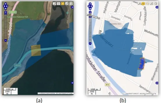
segment the raw data using a spatial tool and then the processed results are visualised through the 235
GLIMPSE WebGL viewer, as shown in Figure2.
Figure 2.User defined (a) LiDAR section polygon represented in orange and (b) processed results in the WebGL viewer.
236
In Section3.1, we detail how spatial hierarchies are built and defined in the GLIMPSE system, 237
while in Section3.2, we describe the optimal approach to data segmentation, fusion and retrieval. 238
Through these sections, the cloud-application based User Interface (UI) in the GLIMPSE system is also 239
detailed that enables interaction, understanding and visualisation of the platforms objectives. 240
3.1. GLIMPSE Spatial Hierarchy 241
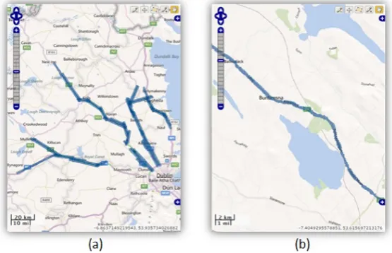
We implemented a 2D spatial hierarchy, where all the spatial data sources from MLS, ALS and 242
terrestrial surveys are stored at different levels of spatial detail. This stage does not change the original 243
spatial detail of the LiDAR but allows a user to evaluate and thus process the available LiDAR in 244
shown in the Google maps UI as blue transparent polygon. In Figure3(a), the coverage of ALS survey
Figure 3.Approximated coverage zone for (a) ALS and (b) MLS datasets.
246
containing 1,700 million points is shown, while Figure3(b) shows the LiDAR coverage of MLS survey 247
consisting of 400 million points. Within the GLIMPSE UI, the user can use standard GIS point and 248
polygon creation tools to intersect a planar view of the available data in this area, which is presented 249
in Section3.2. This is also true for automated process that can be scripted into the GLIMPSE platform. 250
The spatial hierarchy procedure has been implemented as a bespoke implementation of the 251
PostGIS2 ST_ConcaveHull method. This approach was chosen as it presented significant performance 252
improvements over the default PostGIS implementation. This was important, not only because the 253
quantities of LiDAR being processed are so large, but also because the three different LiDAR data source 254
types have very different point density properties. For example, MLS data can have a point density 255
in excess of 4,000 points perm2, where point densities reduce as a function of distance orthogonal to 256
the survey vehicles direction of operation. Effectively this LiDAR data source produces a very dense 257
and detailed route corridor point cloud. On the other hand ALS data, which can also be presented in 258
a corridor like fashion representing the aerial vehicles flight path, the point densities are very much 259
uniform across the scan area and typically in the order of 10 points perm2. 260
The first stage in our process is to snap all the LiDAR data to a spatial grid. A sub-step in the 261
first stage involves the application of a sub-sampling threshold to the LiDAR. This sub-sampling is 262
applied differently depending on the LiDAR data source; in the case of MLS data, areas with high point 263
densities, close to the survey vehicle, are sub-sampled with a higher threshold than areas with lower 264
point densities. The second stage is to generate concave hulls for all the sub-sampled and gridded data. 265
Finally, a spatial union is performed on all the concave hulls for the LiDAR data being processed. 266
This final stage can take the form of a number of different spatial unions such that the highest 267
accuracy concave hull is a direct 2D spatial representation of a single table of raw LiDAR. This idea 268
follows through to unions that define all the data in different spatial configurations; local, regional, 269
national, etc. The spatial union can also be applied in a number of other ways such as modelling the 270
data using the survey based approach that exists in typical commercial software suites. 271
3.2. GLIMPSE Spatial Segmentation & Fusion 272
Having approached each stage of this framework pipeline with a spatial constraint perspective to 273
the fore, it is possible at this stage to optimize the LiDAR data being output. This can be achieved, 274
once again, through procedures that leverage the power of the PostGIS platform through its numerous, 275
generated for the LiDAR, it is relatively easy to highlight use cases which generate bespoke LiDAR 277
subsets from our 29 billion points stored in a 4.2 TB database. 278
These use-cases could be in any relevant form where the process being initiated needs access to 279
LiDAR. Consequently, this could be an automated processing algorithm, such as the road median 280
extraction algorithm, where subsets of LiDAR can be spatially optimized and fused such that the 281
algorithm handles only relevant LiDAR in the system. In Figure3, we can see a sample of the GLIMPSE 282
UI which highlights how this can happen. Alternatively, this example use-case could just as easily be a 283
LiDAR awareness approach where LiDAR can be quickly and easily segmented for a user to view the 284
outputs such that they are suitable for a given process or requirement. 285
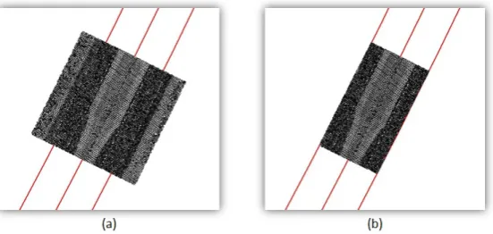
In this example both point or polygon spatial-constraint geometries can be created by a user; 286
polygons have been created in this case as can be seen in Figure 4. This operation provides
Figure 4. User initiated sectioning of (a) and (b) LiDAR datasets with polygon tools for feature extraction processing.
287
the geographical context for the LiDAR query where the user can choose between a 2D or 3D 288
implementation. Either choice will result in a 3D LiDAR point cloud being returned. However, 289
in the 3D case the extra altitude (Z) parameter is added to the spatial query and can be used to bind 290
the point-cloud in the Z domain, i.e. a road median extraction algorithm will not require data outside 291
the boundary of the road surface. These optimizations can significantly reduce the number of points 292
returned which subsequently decreases the query time, required processing time and the rendering 293
time. 294
Extending on from this example is the possibility of numerous different user or process driven 295
use-cases that may require the spatially segmented LiDAR data to be returned based on attribute 296
constraints as well. For every independent LiDAR attribute, including the table’s primary key, an 297
index exists such that searching any LiDAR table becomes a function of the index being searched 298
and not a dependent process on the table’s primary key. Thus, in the previous example we could 299
further constrain the returned point cloud data by requesting only points whose intensity values fall 300
within a certain range, which allows us to continue to leverage the power of the database. Using the 301
optimizations that are inherent to the PostgreSQL database, a standard spatial query will optimize 302
its search based on the spatial index and the primary key of the table. For queries that extend such 303
a search, based on other attributes, the primary key element is easily replaced with the index of the 304
chosen constraint. In the main, runtimes on these attribute constrained queries will be comparable in 305
the single constraint case, although as the number of attribute constraints increases runtimes would 306
logically extend. In the next section, we describe our point cloud retrieval and road median extraction 307
4. Algorithm 309
We developed algorithms to efficiently retrieve ALS data from the GLIMPSE system based on user 310
specified spatial extent and then to automatically extract road median from the retrieved data. The use 311
of GLIMPSE system facilitates the segmentation and fast retrieval of point cloud data for a particular 312
geographical area. In the first part, we describe a method to efficiently retrieve ALS data from the 313
GLIMPSE system based on user specifications while in the second part, an algorithm to automatically 314
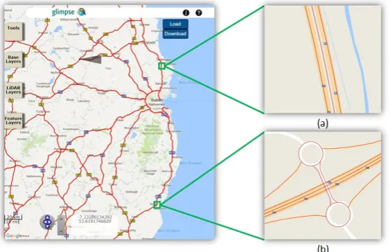
extract road median from the retrieved ALS data is presented. We use road vector polylines in our 315
algorithm as a secondary data source, which were obtained from the National Roads Authority (NRA) 316
in Ireland. These road polylines were imported in the GLIMPSE system, while representing centre, 317
left-lane and right-lane of the dual carriageways in Ireland as shown in Figure5. Each road polyline
Figure 5. Road vector polylines represented in red in the GLIMPSE system, with inset pictures representing (a) N01 and (b) N11 road sections in detail.
318
was associated with Route ID, Road Number, Direction, Section Number and Lane Representation. 319
4.1. Point Cloud Retrieval 320
Our point cloud retrieval algorithm is developed based on the assumption that a polygon spatial 321
tool in the GLIMPSE system can be utilised to segment the ALS data, as shown in Figure6. The
Figure 6.GLIMPSE polygon spatial tool.
322
spatial tool requires height and width parameters along with heading and position (i.e. latitude and 323
longitude) information at the centre of polygon for enabling it to segment the LiDAR data. The user 324
specifies the cross-section length (i.e. height),lcand width,wcdimensions of polygon along with the 325
required total length,lt. The central position and heading parameters of each polygon segment are 326
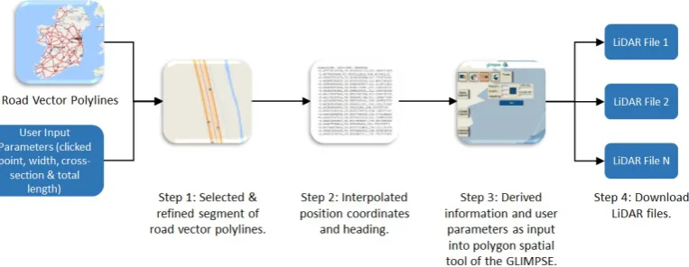
estimated using road vector polylines based on user clicked location. A workflow of the point cloud 327
Figure 7.Point cloud retrieval algorithm.
The user explores the road polylines incorporated in the Google maps UI of GLIMPSE system 329
and can click any point near the preferred road section for which the ALS data is required. In Step 330
1 of our algorithm, the road polyline point nearest to the user clicked location is selected using a 331
kd-tree approach. The k-d tree is a data structure which is used to organise the points in a space with 332
k-dimensions. Each node of a tree specifies an axis and splits the set of points based on whether their 333
coordinate along that axis is greater or less than a node value [48]. The splitting is done based on the 334
first dimension axis and then each level down the division is done based on the next dimension. The 335
splitting points are selected to ensure that the cells do not become long and thin. In our approach, all 336
the road polyline points, representing the centre of the dual carriageway, are split in three dimension 337
and then the polyline point nearest to the user clicked location is selected. The selected polyline point 338
is used to further select the consecutive polyline points based on total length specified by the user. 339
In step 2 of our algorithm, the central position coordinates of each cross-section length are linearly 340
interpolated from the selected road polyline points. The heading at each centre location is derived 341
by first estimating the slope angle from the interpolated position coordinates and then estimating 342
the angle with respect to the North direction. In step 3 of the point cloud retrieval algorithm, the 343
position coordinates and heading information along with user specified length and width dimensions 344
are input into the polygon spatial tool of the GLIMPSE system. The input information facilitates the 345
segmentation of ALS data using the polygon tool and allows the user to download the segmented data 346
from the GLIMPSE system in step 4 of our algorithm. For example, if the user wants to access the ALS 347
data of 2km road section with 100m cross-section length, then 20 data files will be downloaded from 348
the GLIMPSE system. 349
4.2. Road Median Extraction 350
The ALS data files accessed using the point cloud retrieval algorithm are further used to extract 351
the road median. Our road median extraction algorithm is based on the fact that LiDAR elevation and 352
intensity attributes can be efficiently utilised to extract the median [49]. We inputnnumber of ALS 353
data files and road vector polylines in our road median extraction algorithm. The input data files are 354
batch processed to extract continuous road median along the tested road section. The dimensions (i.e. 355
length, width, height) of data section in each file are based on user input parameters in the point cloud 356
retrieval algorithm. A workflow of the road median extraction algorithm is shown in Figure8. In the 357
following sections, we describe various processing steps involved in our algorithm. 358
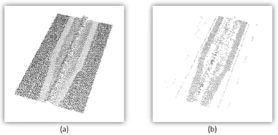
4.2.1. Road Surface Estimation 359
In Step 1 of our algorithm, we use the road vector polylines to estimate the LiDAR points 360
Figure 8.Road median extraction algorithm.
find their intersection with the convex hull fitted to the input LiDAR points. The intersected boundary 362
points are then used to remove the outside points, while inner points are retained which belong to 363
the road surface. Thus, the use of road polylines is efficient in terms of reducing the search space in 364
LiDAR data for extracting the road median. The process of estimating road surface points using road 365
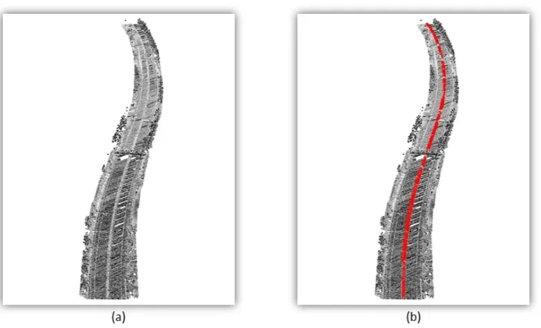
polylines is shown in Figure9.
Figure 9. The input (a) road section points and (b) road surface points estimated using polylines represented in red.
366
4.2.2. Frequency Distribution Analysis 367
The road sections consist of highways crossing above them at some locations, which are required 368
to be removed in order to get a correct estimation of the road median. In Step 2 of our algorithm, these 369
crossing highways are removed based on frequency distribution of the elevation values obtained from 370
the road surface LiDAR points. We assume that along the road section, a large number of LiDAR points 371
will belong to its surface, while in comparison less points will correspond to any highway crossing 372
above it. Based on this assumption, frequency distribution of elevation values is estimated and then 373
elevation value with maximum frequency is identified ashr, which belongs to the road surface. The 374
are retained for further processing. The value ofeparameter is estimated empirically and fixed for 376
all the road sections in such a way that it could be useful in removing the crossing highways. In this 377
way, crossing highways above the road sections are removed by detecting the road surface points with 378
maximum elevation frequency. An example of removing crossing highway above the road section is 379
shown in Figure10.
Figure 10. The road surface (a) with highway crossing above it, which is then (b) removed using frequency distribution analysis.
380
4.2.3. Threshold Analysis 381
In Step 3 of our algorithm, we apply threshold to elevation and intensity attributes in order to 382
get an initial estimation of the road median. The elevation and intensity values are normalised with 383
respect to their minimum and maximum values, and converted to an 8-bit data type. This enables a 384
two way transformation between the 8-bit values and their original LiDAR values, which in turn will 385
allow for the use of a single threshold value for all road sections. We applyTelevandTintthreshold 386
parameters to road surface LiDAR points and get initial road median points, as shown in Figure 4. 387
The values of these threshold parameters are estimated empirically and fixed for all the road sections, 388
which allows for their fully automated application.
Figure 11.Threshold values applied to the (a) road surface points in order to get an initial estimation of the (b) road median.
389
4.2.4. 2D Raster Surface Generation 390
In Step 4 of our algorithm, we generate 2D intensity raster surfaces from the initial estimated road 391
median points using a cell size, c parameter. The value of c is selected based on an average spacing of 392
LiDAR points. The value of each cell in the raster surface is estimated as the average of the intensity 393
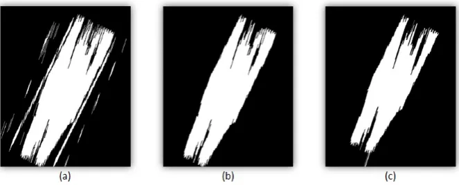
4.2.5. Morphological Operations 395
The initial estimated road median may be incomplete and contain other road surface elements that 396
are introduced through the use of thresholding. To overcome this, we use morphological operations 397
based knowledge analysis of road median in Step 5 of our algorithm [40]. This analysis involves three 398
processes. In the first process, the intensity raster surface is converted into a binary image and then 399
the morphological dilation operation is applied in which a structuring element is placed over the 400
image cells. The purpose of dilation is to use the structuring element to grow cells with a value of 401
1 in order to fill in any holes. A structuring element consists of a binary matrix that represents the 402
selected shape and size. A central element of the matrix represents an origin and the elements with a 403
value of 1 describe a neighbourhood of the structuring element. The origin of the structuring element 404
is positioned over each cell in the binary raster surface to dilate that cell along the neighbourhood of 405
the structuring element. 406
We select a linear shaped structuring element to dilate the cells due to linear pattern of the road 407
median. The length,l, of the linear element is selected empirically and is fixed for all the road sections, 408
which allows us to automate the morphological operation in our algorithm. The linear element is used 409
with aθangle that is calculated from the mean heading of the road polyline points. This angle is useful 410
in dilating the road median cells along the longitudinal direction. The use of dilation operation fills the 411
holes and completes the shapes of road median in the input binary image. An example of the dilation 412
of input binary image using linear element is shown in Figure12(a).
Figure 12.Morphological operations based knowledge analysis: (a) dilated image, (b) road surface cells removed and (c) eroded image.
413
In the second process, we group cells into objects in the dilated image using connectivity. If a cell 414
has a value of 1 then it is connected to the cells whose values are 1 and are directly above, below, left or 415
right of that cell. We calculate the length and average width values of each object in the dilated image. 416
Objects whose length and average width values are less than length threshold,TLand width threshold, 417
TWare considered as other road surface elements and are removed from the image, as shown in Figure 418
12(b). These length and width threshold values are estimated based on knowledge about standard 419
dimensions of the road median. In the third process, we apply an erosion operation to the dilated 420
image in order to retain the original boundary shape of the road median. In an erosion operation, cells 421
are removed from the road median cells using a structuring element. The linear shaped structuring 422
element used for dilation is also applied to erode the road median cells, as shown in Figure12(c). In 423
this way, the combined use of morphological operations and knowledge about the dimensions of the 424
road median is able to complete its shape and remove other road surface elements. 425
4.2.6. 3D Road Median Points 426
In final Step 6 of our algorithm, we extract the 3D road median points from the 2D output. The 427
original 3D LiDAR points which are contained within the 2D road median cell boundaries are extracted. 428
5. Experimentation 430
The dataset acquired using an ALS system along dual carriageway roads in Ireland was uploaded 431
into the GLIMPSE system. In the first part, we applied our point cloud retrieval algorithm to efficiently 432
access ALS data from the GLIMPSE system based on our specific requirements. We, as a user, explored 433
the road polylines imported in the GLIMPSE system and clicked the points near two preferred road 434
sections of dual carriageway. In each section, other input parameters were provided aslc = 50m, 435
wc = 50m andlt = 1000m. The first 1km section consisted of road median with narrow concrete 436
barrier, as shown in Figure13(a), while the second 1km section contained road median with wide 437
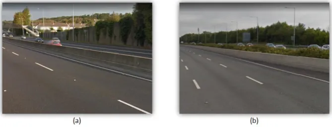
grass-hedge concrete barrier, as shown in Figure13(b).
Figure 13.Digital images of the (a) first road section with narrow concrete barrier and the (b) second road section with wide grass-hedge barrier. (Geographic locations: (a) 53021011”N 6027026.1”W (b) 5302609.8”N 6012037.7”W) (Images Courtesy: Streetview, Google)
438
The selected road polyline points and input parameters were used to estimate the central position 439
and heading information of each cross-section length along the two road sections. Finally, the derived 440
information facilitated the downloading of ALS data files from GLIMPSE in accordance with the 441
specified parameters. In each 1km road section,n=20 number of data files were accessed with each 442
corresponding to 50m cross-section length. 443
In the second part, the accessed data files were batch processed to extract the road median 444
along the tested road sections using empirically estimated parameters. The value ofewas selected 445
as 4m, which was found to be useful in removing the highways crossing above the road sections. 446
The threshold parameters,TelevandTintwere applied as 200 and 100 respectively, to get an initial 447
estimation of road median in both the sections. The cell size,c=0.1 was used to generate 2D intensity 448
raster surface from initial estimated road median points. The length,l of linear element was used 449
as 50, while angleθwas calculated from the mean heading of the road polyline points. The length 450
threshold,TLwas applied as 100 in both the road sections, however due to different width size of 451
median, we applied different values ofTWin them. The value ofTWwas provided as 5 in the first road 452
section, while in the second section it was applied as 10. The final extracted road median in the first 453
and second road sections are shown in Figures14and15respectively. In the next section, we present 454
the validation of experimental results and discuss them. 455
6. Results & Discussion 456
Our algorithms were able to successfully extract the road median in the tested road sections based 457
on a specified spatial extent. We, as a user, specified input parameters in the point cloud retrieval 458
algorithm to efficiently access the ALS data for a particular geographical area from a large volume of 459
data stored in the GLIMPSE system. The retrieved datasets were further processed to automatically 460
extract the road median along the tested road sections. We validated the extracted road median in 461
the first and second road sections using a manually digitised road median. Our validation approach 462
Figure 14.The (a) ALS point cloud along the first road section and the (b) extracted road median points represented in red.
edges from their corresponding manually digitised road median points [39]. In our approach, we 464
utilised the centre road polyline point which was selected at 2m intervals along the road section in 465
each iteration. The extracted and digitised road median points were rotated toward the horizontal 466
X-axis based on heading angle of the selected road polyline point. This horizontal rotation was done to 467
simplify the process of estimating orthogonal distance. After rotation, linear splines were fitted to both 468
the 2D-extracted and digitised road median points. The purpose of the spline fitting was to facilitate 469
the interpolation of Y-axis values of the extracted and digitised road median points with respect to 470
the known X-axis value of the selected road polyline point. Finally, we calculated an orthogonal 471
Euclidean distance between the extracted and digitised road median points, which were rotated 472
toward the horizontal X-axis. The positive or negative value indicated the inside or outside position of 473
the extracted road median point with respect to the digitised road median point. This process was 474
iterated for all the road polyline points selected at a 2m interval. Thus, the orthogonal distance was 475
used to estimate the accuracy of extracted median in the two tested road sections. Box plots for the 476
accuracy values of extracted road median points along left and right edges in the first and second road 477
sections are shown in Figures16and17respectively. We also carried out statistical analyses of the 478
accuracy values of extracted road median points along left and right edges in the first and second road 479
sections as shown in Table1. 480
Our road median extraction algorithm was able to successfully extract the road median in the 481
first and second road sections. In the first road section, the accuracy values were found to be better 482
than in the second road section. The minimum-maximum range values were lowest in the first section, 483
while its accuracy values along the left and right edges were within a±2m tolerance. In the second 484
road section, 10.16% and 1.39% accuracy values along the left and right edges respectively were more 485
than±2m tolerance. Similarly, the mean, median and RMSE values in the first road section were 486
found to be better than in the second road section. This was due to higher reflectivity obtained from 487
the narrow concrete barrier in the first road section than from the grass-hedge concrete barrier in the 488
second section. The non-continuous shapes of some road median also contributed to lower accuracy 489
values in the second road section as shown in Figure18. In both the road sections, the road median 490
Figure 15.The (a) ALS point cloud along the second road section and the (b) extracted road median points represented in red.
road sections, the accuracy values of road median points along the right edge were higher within 492
±0.2m,±0.5m,±1m and±2m tolerances than along the left edge. 493
Our automated algorithm extracted the road median with an average RMSE values of 0.55m 494
and 0.92m in the first and second road sections respectively. This low accuracy was attributed to the 495
fact that road median at some locations along the tested road sections were missed, while at other 496
locations, the adjacent lane markings were included in the output as false positives. High reflectivity 497
from the lane markings led to their inclusion in the initial estimated road median during threshold 498
applied to the intensity attribute. Further, their close proximity to road median did not enabled their 499
removal during morphological operations. The value of LiDAR intensity attribute depends upon 500
incidence angle of the laser pulse, the distance from the laser scanner and the illuminated surface. 501
The normalisation of intensity attribute with respect to these factors will provide true reflectance 502
values from the targeted objects. The use of such normalised intensity values in our algorithm will 503
improve the quality of extracted road median. The tested road sections were also associated with 504
highways crossing above them at some locations, which were efficiently removed based on frequency 505
distribution analysis of elevation values. This analysis was done based on an assumption that large 506
number of points will belong to the road surface in comparison with crossing highways. However, in 507
case of wider highway, the large number of LiDAR points will belong to it and this will lead to the 508
removal of road section beneath it. In the morphological operations, we applied different values of 509
width threshold due to different width of the median in the tested road sections. 510
We analysed the computational performance of our two algorithms by estimating the total time 511
taken to retrieve the data from the GLIMPSE system and then to finally extract the road median. 512
In the first and second road sections with each 1km length and 50m cross-section length, it took 513
approximately 37 minutes and 119 minutes respectively to retrieve and process the dataset. This 514
analysis was performed on a computer with Intel Core i5-6600 processor @3.30GHz, 8GB RAM and a 515
64-bit operating system. The second road section consisted of wider road median due to which it took 516
more time to process the dataset in comparison with the first road section. 517
7. Conclusion 518
In this paper, we presented the GLIMPSE system that provides a comprehensive framework 519
Figure 16.Box plot for the accuracy values of extracted road median points along left and right edges in the first road section.
Figure 17.Box plot for the accuracy values of extracted road median points along left and right edges in the second road section.
Table 1.Statistical analysis of the accuracy values of extracted road median points along left and right edges in the first and second road sections.
First Section Second Section
Left Right Left Right
minimum (m) -0.93 -1.48 -3.18 -0.36
maximum (m) 1.49 1.24 0.26 2.34
lower adjacent (m) -0.93 -1.28 -2.93 -0.36
upper adjacent (m) 1.49 0.91 0.26 1.26
25th percentile (m) -0.27 -0.47 -1.49 0.24
75th percentile (m) 0.49 0.09 -0.36 0.67
mean (m) 0.17 -0.20 -0.93 0.51
median (m) 0.25 -0.25 -0.64 0.41
inside±0.2m (%) 15.66 23.69 9.47 19.40
inside±0.5m (%) 57.63 69.08 38.57 60.28
inside±1m (%) 92.17 94.18 63.05 89.38
inside±2m (%) 100 100 89.84 98.61
outside±2m (%) 0 0 10.16 1.39
Figure 18.The (a) ALS point cloud with some non-continuous road median along the second road section and their (b) extraction represented in red.
representation of large scale data in a geographical meaningful way, that enables the user to spatially 521
segment the data based on its requirement. The use of such a system provides a framework for the fast 522
retrieval of point cloud data based on an optimal spatial extent which, in turn, improves the efficiency 523
of automated algorithms in terms of computational cost and reduced processing. We developed the 524
methods to efficiently retrieve point clouds from the GLIMPSE system and to automatically extract the 525
road median from the retrieved data. In our point cloud retrieval algorithm, the road vector polylines 526
are used as secondary data source to estimate the parameters required for spatial segmentation of ALS 527
point cloud in the GLIMPSE based on user input information. In case of MLS dataset, the navigation 528
points can also be utilised as secondary data source, which are usually procured during the data 529
acquisition process. The GLIMPSE system provides a single platform for storage, integration, retrieval 530
and processing of large volume of LiDAR point cloud in a computationally efficient manner. 531
Our road median extraction algorithm was developed based on the assumption that LiDAR 532
data provides elevation and intensity values, which can be utilised to distinguish the median. The 533
use of road polylines enables to estimate the points belonging to the road surface, which in turn 534
facilitates more accurate extraction of road median. We then perform the frequency distribution 535
analysis of elevation values, which provides for the removal of the highways crossing above the road 536
sections. The morphological operations based knowledge analysis is useful in completing the shape of 537
the road median and removing other road surface elements, that are introduced through the use of 538
thresholding. The algorithms were tested on two road sections to extract the concrete and grass-hedge 539
based road medians. The successful extraction of road median from these multiple road section 540
environments based on user requirement validates our two algorithms. The developed workflow can 541
assist authorities in ensuring rapid and timely maintenance of road features along the route corridor 542
environment. 543
In future work, the road median algorithm will be tested on road sections with more distinct 544
medians. The elevation and intensity threshold values applied to get an initial estimate of the road 545
median, were estimated empirically. However, a more robust and automated approach will need to be 546
developed in order to get the threshold values. We will also focus on the normalisation of the intensity 547
attribute, which will improve the quality of road median extraction. The size of input data sections 548
and cell size of raster surfaces impact the efficiency of our algorithm in terms of computational cost. 549
These parameters are required to be efficiently analysed to find their optimal values. Future work 550
will also focus on the integration of LiDAR and imagery data acquired from multiple platforms in the 551
GLIMPSE system, which will then be utilised to develop other road feature extraction algorithms. 552
Acknowledgments:Research presented in this paper was initially funded by the Irish Research Council Enterprise 553
under the National Development Plan. This research also received financial support through Science Foundation 555
Ireland grant SFI 13/IF/I2782. The research was continued at Centre Tecnològic de Telecomunicacions de 556
Catalunya (CTTC/CERCA), Barcelona. The authors gratefully acknowledge this support. 557
Author Contributions:Pankaj Kumar collaborated with Paul Lewis and Conor P. McElhinney in developing the 558
concept and performing the experiments. Pankaj Kumar and Paul Lewis contributed in preparing this manuscript. 559
Conflicts of Interest:The authors declare no conflict of interest. 560
Abbreviations 561
The following abbreviations are used in this manuscript: 562
563
LiDAR Light Detection and Ranging MLS Mobile Laser Scanning ALS Airborne Laser Scanning
GLIMPSE Global LiDAR and Imagery Mobile Processing Spatial Environment DEM Digital Elevation Model
TIN Triangulated Irregular Network SDBMS Spatial Database Management System MBR Minimum Bounding Rectangle MBB Minimum Bounding Boxes DTM Digital Terrain Model UI User Interface
NRA National Roads Authority 564
References 565
1. Darnel, C. Using LiDAR to solve industry challenges.Geoconnexion International Magazine2012,11, 18–19. 566
2. Kumar, P. Road features extraction using terrestrial mobile laser scanning system. Ph.d., National 567
University of Ireland Maynooth (NUIM), 2012. 568
3. Rutzinger, M.; Elberink, S.J.O.; Pu, S.; Vosselman, G. Automatic extraction of vertical walls from mobile 569
and airborne laser scanning data.The International Archives of the Photogrammetry, Remote Sensing and Spatial 570
Information Sciences, 1-2 September, Paris, France2009,XXXVIII-3, 7–11. 571
4. Kumar, P.; McElhinney, C.P.; Lewis, P.; McCarthy, T. An automated algorithm for extracting road edges 572
from terrestrial mobile LiDAR data. ISPRS Journal of Photogrammetry and Remote Sensing2013,85, 44–55. 573
5. Kumar, P.; Lewis, P.; McElhinney, C.P. Parametric analysis for automated extraction of road edges from 574
mobile laser scanning data. ISPRS Annals of the Photogrammetry, Remote Sensing and Spatial Information 575
Sciences, 28-30 October, KualaLumpur, Malaysia2015,II-2/W2, 215–221. 576
6. Chen, Q. Airborne LiDAR data processing and information extraction. Photogrammetric Engineering & 577
Remote Sensing2007,73, 109–112. 578
7. Yang, B.; Dong, Z.; Zhao, G.; Dai, W. Hierarchical extraction of urban objects from mobile laser scanning 579
data. ISPRS Journal of Photogrammetry and Remote Sensing2015,99, 45–57. 580
8. Lewis, P.; McElhinney, C.P.; Schon, B.; McCarthy, T. Mobile mapping system LiDAR data framework. 581
The International Archives of the Photogrammetry, Remote Sensing and Spatial Information Sciences 2010, 582
XXXVIII-4, 135–138. 583
9. Lewis, P.; McElhinney, C.P.; McCarthy, T. LiDAR data management pipeline; from spatial database 584
population to web-application visualization. 3rd International Conference on Computing for Geospatial 585
Research and Applications, 1-3 July, Washington, USA2012. 586
10. Cabo, C.; Ordonez, C.; Garcia-Cortes, S.; Martinez, J. An algorithm for automatic detection of pole-like 587
street furniture objects from mobile laser scanner point clouds. ISPRS Journal of Photogrammetry and Remote 588
Sensing2014,87, 47–56. 589
11. Ming, G.; Yanmin, W.; Youshan, Z.; Junzhao, Z. Research on database storage of large-scale terrestrial 590
LiDAR data. International Forum on Computer Science-Technology and Applications, 25-27 December, Chongqing, 591
China2009, pp. 19–23. 592
12. Bruenig, M.; Zlatanova, S. 3D Geo-DBMS. Directions Magazine (Available: 593
13. Schon, B.; Bertolotto, M.; Laefer, D.F.; Morrish, S.W. Storage, manipulation and visualization of LiDAR 595
data. The International Archives of the Photogrammetry, Remote Sensing and Spatial Information Sciences, 25-28 596
Febraury, Trento, Italy2009,XXXVIII-5, 8. 597
14. Guttman, A. R-trees: a dynamic index structure for spatial searching. ACM SIGMOD International 598
Conference on Management of Data, 18-21 June, Boston, USA1984,14, 47–57. 599
15. Samet, H.Foundations of multidimensional and metric data structures; Morgan Kaufmann Publisher, 2006; p. 600
1024. 601
16. Agarwal, P.K.; Arge, L.; Danner, A., From Point Cloud to Grid DEM: A Scalable Approach. InProgress in 602
Spatial Data Handling: 12th International Symposium on Spatial Data Handling; Riedl, A.; Kainz, W.; Elmes, 603
G.A., Eds.; Springer Berlin Heidelberg, 2006; pp. 771–788. 604
17. Hua, L.; Zhengdong, H.; Qingming, Z.; Peng, L. A database approach to very large LiDAR data 605
management. The International Archives of the Photogrammetry, Remote Sensing and Spatial Information 606
Sciences, 3-11 July, Beijing, China2008,XXXVII, 463–468. 607
18. Stal, C.; Maeyer, P.D.; Wulf, A.D.; Nuttens, T.; Vanclooster, A.; Weghe, N.V.D. An optimized workflow 608
for processing airborne laser scan data in a GIS-based environment. The International Archives of the 609
Photogrammetry, Rempote Sensing and Spatial Information Sciences, 3-4 November, Berlin, Germany2010, 610
XXXVIII, 163–167. 611
19. Nandigam, V.; Baru, C.; Crosby, C. Database design for high-resolution LiDAR topography data. 612
International Conference on Scientific and Statistical Database Management, 30 June-2 July, Heidelberg, Germany 613
2010,1, 151–159. 614
20. Hongchao, M.; Wang, Z. Distributed data organization and parallel data retrieval methods for huge laser 615
scanner point clouds.Computers & Geosciences2011,37, 193–201. 616
21. Elseberg, J.; Borrmann, D.; Nüchter, A. One billion points in the cloud - an octree for efficient processing of 617
3D laser scans. ISPRS Journal of Photogrammetry and Remote Sensing2013,76, 76–88. 618
22. Cura, R.; Perret, J.; Paparoditis, N. A scalable and multi-purpose point cloud server (PCS) for easier and 619
faster point cloud data management and processing. ISPRS Journal of Photogrammetry and Remote Sensing 620
2017,127, 39–56. 621
23. NSF. OpenTopography - LiDAR access facility. http://opentopo.sdsc.edu/datasets?listAll=true2017. 622
24. Dielmo. LiDAR-Online. http://www.lidar-online.com/tools/maps/?lang=en2017. 623
25. Clode, S.; Kootsookos, P.; Rottensteiner, F. The automatic extraction of roads from LiDAR data. The 624
International Archives of the Photogrammetry, Remote Sensing and Spatial Information Sciences, 12-23 July, 625
Istanbul, Turkey2004,XXXV, 231–236. 626
26. Vosselman, G.; Liang, Z. Detection of curbstones in airborne laser scanning data. The International Archives 627
of the Photogrammetry, Remote Sensing and Spatial Information Sciences, 1-2 September, Paris, France2009, 628
XXXVIII, 111–116. 629
27. Hu, X.; Tao, C.V.; Hu, Y. Automatic road extraction from dense urban area by integrated processing of 630
high resolution imagery and lidar data. The International Archives of the Photogrammetry, Remote Sensing and 631
Spatial Information, 12-23 July, Istanbul, Turkey2004,XXXV, 320–324. 632
28. Mumtaz, S.A.; Mooney, K. A semi-automatic approach to object extraction from a combination of image 633
and laser data. The International Archives of the Photogrammetry, Remote Sensing and Spatial Information 634
Sciences, 3-4 September, Paris, France2009,38, 53–58. 635
29. Elberink, S.J.O.; Vosselman, G. 3D information extraction from laser point clouds covering complex road 636
junctions.The Photogrammetric Record2009,24, 23–36. 637
30. Li, Y.; Yong, B.; Wu, H.; An, R.; Xu, H. Road detection from airborne LiDAR point clouds adaptive for 638
variability of intensity data.Optik - International Journal for Light and Electron Optics2015,126, 4292–4298. 639
31. Hui, Z.; Hu, Y.; Jin, S.; Yevenyo, Y.Z. Road centerline extraction from airborne LiDAR point cloud based on 640
hierarchical fusion and optimization.ISPRS Journal of Photogrammetry and Remote Sensing2016,118, 22–36. 641
32. Ferraz, A.; Mallet, C.; Chehata, N. Large-scale road detection in forested mountainous areas using airborne 642
topographic lidar data.ISPRS Journal of Photogrammetry and Remote Sensing2016,112, 23–36. 643
33. Boyko, A.; Funkhouser, T. Extracting roads from dense point clouds in large scale urban environment. 644
ISPRS Journal of Photogrammetry and Remote Sensing2011,66, S2–S12. 645
34. Zhou, L.; Vosselman, G. Mapping curbstones in airborne and mobile laser scanning data. International 646
35. Serna, A.; Marcotegui, B. Urban accessibility diagnosis from mobile laser scannning data. ISPRS Journal of 648
Photogrammetry and Remote Sensing2013,84, 23–32. 649
36. Yang, B.; Fang, L.; Li, J. Semi-automated extraction and delineation of 3D roads of street scene from mobile 650
laser scanning point clouds.ISPRS Journal of Photogrammetry and Remote Sensing2013,79, 80–93. 651
37. Wang, H.; Luo, H.; Wen, C.; Cheng, J.; Li, P.; Chen, Y.; Wang, C.; Li, J. Road boundaries detection based 652
on local normal saliency from mobile laser scanning data. IEEE Geoscience and remote sensing letters2015, 653
12, 2085–2089. 654
38. McElhinney, C.P.; Kumar, P.; Cahalane, C.; McCarthy, T. Initial results from european road safety inspection 655
(EURSI) mobile mapping project.The International Archives of Photogrammetry, Remote Sensing and Spatial 656
Information Sciences, 21-24 June, Newcastle, UK2010,XXXVIII, 440–445. 657
39. Kumar, P.; Lewis, P.; McElhinney, C.P.; Boguslawski, P.; McCarthy, T. Snake energy analysis and result 658
validation for a mobile laser scanning data based automated road edge extraction algorithm.IEEE Journal 659
of Selected Topics in Applied Earth Observations and Remote Sensing2017,10, 763–773. 660
40. Kumar, P.; McElhinney, C.P.; Lewis, P.; McCarthy, T. Automated road markings extraction from mobile 661
laser scanning data.International Journal of Applied Earth Observation and Geoinformation2014,32, 125–137. 662
41. Guo, J.; Tsai, M.J.; Han, J.Y. Automatic reconstruction of road surface features by using terrestrial mobile 663
lidar. Automation in Construction2015,58, 165–175. 664
42. Teo, T.A.; Chiu, C.M. Pole-like road object detection from mobile LiDAR system using a coarse-to-fine 665
approach. IEEE Journal of Selected Topics in Applied Earth Observations and Remote Sensing2015,8, 4805–4818. 666
43. Yan, W.Y.; Morsey, S.; Shaker, A.; Tulloch, M. Automated extraction of highway light poles and towers 667
from mobile LiDAR data. Optics & Laser Technology2016,77, 162–168. 668
44. Kumar, P.; Lewis, P.; McElhinney, C.P.; Abdul-Rahman, A. An algorithm for automated estimation of road 669
roughness from mobile laser scanning data.The Photogrammetric Record2015,30, 30–45. 670
45. Guan, H.; Li, J.; Yu, Y.; Chapman, M.; Wang, H.; Wang, C. Iterative tensor voting for pavement crack 671
extraction using mobile laser scanning data. IEEE Transactions on Geoscience and Remote Sensing2015, 672
53, 1527–1537. 673
46. Diaz-Vilarino, L.; Gonzalez-Jorge, H.; Bueno, M.; Arias, P.; Puente, I. Automatic classification of urban 674
pavements using mobile LiDAR data and roughness descriptors.Construction and Building Materials2016, 675
102, 208–215. 676
47. Rutzinger, M.; Pratihast, A.K.; Elberink, S.O.; Vosselman, G. Detection and modelling of 3D trees from 677
mobile laser scanning data. The International Archives of the Photogrammetry, Remote Sensing and Spatial 678
Information Sciences, 21-24 June, Newcastle, UK2010,XXXVIII, 520–525. 679
48. Maneewongvatana, S.; Mount, D.M. Analysis of approximate nearest neighbor searching with clustered 680
point sets.First Workshop on Algorithm Engineering and Experimentation, 15-16 January, Baltimore, US1999, 681
p. 20. 682
49. Kumar, P.; Lewis, P. Automated extraction of road median from airborne laser scanning data. The 38th 683