Worst-Case Tolerance Synthesis for Low-Sidelobe Sparse
Linear Arrays Using a Novel Self-Adaptive Hybrid
Differential Evolution Algorithm
Tao Ni*, Yong-Chang Jiao, Li Zhang, and Zi-Bin Weng
Abstract—A worst-case tolerance synthesis problem for low-sidelobe sparse linear arrays is solved by using a novel self-adaptive hybrid differential evolution (SAHDE) algorithm. First, we establish a worst-case tolerance synthesis model for low-sidelobe sparse linear arrays, in which random position errors are considered and assumed to obey the Gaussian distributions. Through the random sampling, the random model is converted to a deterministic optimization problem. Then, a novel SAHDE algorithm is presented for solving the problem. As a modification to the existing hybrid differential evolution algorithm, a simplified quadratic interpolation (SQI) operator is used to tune the control parameters self-adaptively, establishing the connections between control parameters and the fitness values. In order to determine appropriate control parameter values quickly, a selection operation is also used. Detailed implementation procedure for the SAHDE algorithm is presented, and some numerical results show its effectiveness. Finally, for the deterministic optimization problem, we present a fast way for calculating its fitness values. The SAHDE algorithm is used to obtain optimal nominal element positions. Simulated results illustrate that the worst-case peak sidelobe levels for the sparse linear arrays are improved evidently. The SAHDE algorithm is efficient for solving the worst-case tolerance synthesis problem.
1. INTRODUCTION
Over the past years, synthesis of unequally spaced arrays has been studied in depth. Compared with periodic arrays, since the array periodicity is broken, unequally spaced arrays have shown several promising characteristics and probably have some potential advantages [1–4]. Specifically, grating lobes can be restrained in this case, and the array may get lower peak sidelobe levels (PSLLs), while the sidelobes of equally spaced arrays with uniform excitation distribution are greater than about−13.4 dB. Furthermore, it is possible to reduce the number of elements in one certain aperture, which helps to reduce the array cost. Recently, the design techniques mainly focus on two kinds of unequally spaced arrays: thinned arrays [5, 28–29], which are derived by exciting some elements in an equally spaced array, and sparse arrays [2, 3, 6–11, 30–31], in which the spacings of elements are random. In the sparse arrays with uniform excitation distribution, the element spacings with more degree of freedom are optimized to gain lower PSLLs, which makes this kind of arrays be studied widely. Practically the element positions of the spares array possess the random errors. However, in the existing research, influence of the element position errors is always neglected. For sparse arrays, the low-sidelobe levels are directly related to position of each element, and presence of the position errors will have a great impact on peak sidelobe levels (PSLLs). Therefore, the tolerance synthesis problem considering random position errors is worth of research.
Received 14 January 2016, Accepted 18 February 2016, Scheduled 1 March 2016
* Corresponding author: Tao Ni (tao [email protected]).
As a pioneering work, Schjaer-Jacobsen [13] studied the worst-case tolerance optimization of linear broadside arrays, by using algorithms for optimum tolerance assignment problems [12]. However, in his algorithms, derivative information is needed. In [14], Jiao et al. studied the worst-case tolerance optimization synthesis for low sidelobe linear arrays by using the regular polyhedron method, a direct local search method. However, a suitable initial value should be provided, and a local optimal solution is obtained. In [15], the interval arithmetic is applied to analyze only impact of the manufacturing tolerances of the excitation amplitudes on the radiated array patterns. In [32], the interval analysis is applied to analyze the pattern tolerances when phase errors exist in the excitation weights. A design of linear arrays in the presence of tolerances on the amplitude weights is optimized by interval analysis and convex optimization in [33]. The linear array’s excitation tolerances are optimized for the robust amplitude beamforming in [34]. However, these works in [33, 34] are designed for array’s excitations and not for sparse array’s position errors. In [16], the tolerable linear arrays are designed by using the genetic algorithm. The tolerance optimization is highly important and computationally difficult [16], so evolutionary algorithms are suitable for solving the problems.
In recent years, evolutionary algorithms, such as genetic algorithm (GA) [5, 6, 9, 23], particle swarm optimization (PSO) [7, 24–27], and differential evolution (DE) [8, 10, 11], are widely used to solve the antenna optimization problem. In [5, 6, 9, 23], GA and modified GA are used to synthesize the thinning array, sparse array, and adaptive array respectively. In [7], PSO is used to synthesis the linear array and control the null location. In [24–26], PSO algorithms are used to optimize a prefractal monopole antenna, broadband nanoplasmonic arrays and multiple band antenna. In [27], PSO algorithm is applied in microwave image. As a population-based stochastic global optimization algorithm, DE has been successfully applied to many optimization problems. In [8], the authors have been presented an overview of DE-based approaches used in electromagnetics, which pointing out that the DE algorithm and its modified algorithm are effective to solve the electromagnetics problem. However, tuning control parameters involved in DE is a challenging task. For tolerance optimization problems, it is certain to cause computationally difficult and waste time by tuning control parameters blindly. In some modified self-adaptive algorithms such as SaDE and jDE [17, 18], the control parameters are self-adapted to gain better optimal results, based on the learning experiences from previous generations. However, these self-adaptive algorithms do not make full use of the fitness values available in their self-adaptive strategies.
Simplified quadratic interpolation (SQI) is a powerful direct search method. In [19–22], the SQI method is used to improve performance of some evolutionary algorithms, such as Price’s algorithm, the genetic algorithm, and the DE algorithm. In [22], Zhang et al. proposed a hybrid differential evolution (HDE) algorithm with the SQI operator to solve complex antenna design problems. However, the self-adaptive technique is not used in [22].
In this paper, inspired by above ideas, we propose a novel self-adaptive hybrid differential evolution (SAHDE) algorithm for solving worst-case tolerance synthesis problem. For the low-sidelobe sparse linear array, taking the nominal element positions as design parameters, a worst-case tolerance synthesis model considering the random position errors is established. The errors are assumed to obey the Gaussian distributions. Sample points are chosen randomly within a fixed position tolerance region, and then the random tolerance synthesis model is converted to a deterministic optimization problem. In order to solve the problem easily, we presented a new self-adaptive parameter control technique, and a novel SAHDE algorithm. In the algorithm, the control parameters (difference scale factor F, and crossover probability factor CR) are produced by the SQI operator, and the connections between control parameters and fitness values available are established. 11 benchmark problems are used to validate effectiveness of the novel algorithm. Moreover, a sparse linear array is optimized to gain lower PSLLs by using the SAHDE algorithm. Simulated results show that the SAHDE algorithm is efficient. Finally, a fast way for calculating fitness values of the deterministic optimization problem is presented. The SAHDE algorithm is used to minimize the worst-case PSLLs and obtain optimal nominal element positions for the low-sidelobe sparse linear array. Simulated results illustrate that the worst-case peak sidelobe levels for the sparse linear arrays are improved evidently.
the SAHDE algorithm and related simulation results are shown in Section 4. Conclusions are drawn in Section 5.
2. MODEL OF WORST-CASE TOLERANCE SYNTHESIS FOR THE LOW-SIDELOBE SPARSE LINEAR ARRAY
Geometry of the symmetrical sparse linear array with isotropic point source element is shown in Fig. 1, where N is the element number, and di represents position of the ith element, i = −M, . . . ,−1,0,1, . . . , M. Define
D= (d−M, . . . , d−1, d0, d1, . . . , dM) (1)
The array pattern of theN-element sparse linear array with uniform excitation is expressed as
E(θ,D) =
M
i=−M
exp(jksinθdi) (2)
wherek= 2π/λis the propagation constant.
When the array is symmetrical and the center element located in the origin of coordinates,d= 0, di =d−i, and the array pattern is expressed as
E(θ,D) = 1 + 2
M
i=1
cos(jksinθdi) (3)
The design objective is to minimize the PSLL value and find the optimal element positions. For this purpose, the fitness function is defined as
f itness0(D) = max
θ∈S
Emax((θ,DE)) (4)
whereSrepresents the sidelobe region corresponding toD. As a constraint condition,dishould satisfy [6]
min{di−dj,0≤j≤i≤M}> dmin (5)
wheredmin is the minimum element spacing of the array.
By minimizing Eq. (4) under constraint of Eq. (5), proper D can be gained. In engineering applications, however, the element position errors always exist, and the random position errors deteriorate the PSLL of the sparse linear array. In the following, taking the nominal element positions as design parameters, a worst-case tolerance synthesis model considering random position errors with fixed tolerance region is established.
Usually, the element positions are symmetrical. However, the element errors may be asymmetrical. Define the actual element position vector as
Da= (da−M, . . . , da−1, da0, da1, . . . , daM) (6)
For every element in Da, we assume that dai obeys the Gaussian distribution with mean di and standard deviation σi
dai ∼N(di, σ2i) (7)
1
d 2d
1 M
d − dM
1 − d 2 − d
Ă
Ă
1
d d2
1)
−(M
d −
−M
d
θ
... ...
Define the position error vector as
Dc= (dc−M, . . . , dc−1, dc0, dc1, . . . , dcM) (8)
dci represents theith element position error,i=−M,−(M −1), . . . ,0, . . . , M−1, M. Actual position coordinate vector Dais expressed as
Da=D+Dc (9)
For every element in Dc, obviously dci obeys the Gaussian distribution with mean 0 and standard deviationσi
dci ∼N(0, σi2) (10)
In Gaussian distribution N(μ, σ), 99.7% data are within interval (μ−3σ, μ+ 3σ), and only 0.3% data are outside. In fact, the 0.3% possibility is extremely small, and it can be ignored. Usually, interval (μ−3σ, μ+ 3σ) is considered instead of all possibilities. So, the tolerance region is defined as
Ω ={Dc| −3σi < dci<3σi, i=−M, . . . , M} (11)
For the N-element sparse linear array with uniform excitation considering the random position errors, the array pattern is expressed as
E(θ,D,Dc) =
M
m=−M
exp[iksinθ(dm+dcm)] (12)
The PSLLs can be calculated by
SLL(D,Dc) = max
θ∈S
E(max(θ,D,EDc) ) (13)
whereSrepresents the sidelobe region corresponding toDandDc. In order to gain better PSLLs, taking the nominal element positionsD as design parameters, the optimization problem can be expressed as
minimize
D SLL(D,Dc) (14)
Since Dc is a Gaussian random vector, Problem (14) is a stochastic optimization problem, and it is difficult to solve Problem (14) directly. In order to solve Problem (14) easily, we randomly choose N S sample points in the tolerance region of Eq. (11)
Dci, i= 1,2, . . . , N S
The optimization task is to minimize the PSLLs for all possible Dc vectors, including the worst-case PSLLs. Thus Problem (14) can be formulated as the multi-objective optimization problem
minimize
D SLL(D,Dci), i= 1,2, . . . , N S (15)
Problem (15) is a multi-objective optimization problem with many objectives, and it is also difficult to solve Problem (15) directly. Usually, if the worst-case PSLL is minimized, the optimization task is reached. We should pay attention to the worst-case PSLLs. Therefore, Problem (15) can be converted to the single-objective optimization problem
minimize
D maximize1≤i≤NS SLL(D,Dci) (16)
The fitness function is expressed as
f itness (D) = maximize
1≤i≤NS SLL(D,Dci) (17)
3. NOVEL SELF-ADAPTIVE HYBRID DIFFERENTIAL EVOLUTION ALGORITHM AND ITS NUMERICAL EXPERIMENTS
3.1. Hybrid Differential Evolution Algorithm
Differential evolution (DE) is a simple powerful population-based stochastic search algorithm. In the HDE algorithm (DESQI for short in [22]), the simplified quadratic interpolation operator is incorporated with DE to accelerate the convergence of DE. The main operations in the HDE algorithm are described as follows.
3.1.1. Initializing Parameters and Population
Initializing parameters, difference scale factor F, crossover probability factor CR, population sizeN P, and original populationX0, X0 = (X1,0, X2,0, . . . , Xi,0, . . . , XNP,0), whereXi,0is aD-dimension vector.
In [22], F = 0.5,CR= 0.9, andN P is chosen based on the specific problem.
3.1.2. Mutation
At Gth generation, Xi,G= (x1,i,G, x2,i,G, . . . , xj,i,G, . . . , xD,i,G). This operation creates the mutant trial
vectorVi,G+1 = (v1,i,G+1, v2,i,G+1, . . . , vj,i,G+1, . . . , vD,i,G+1) based on the current parent populationXG.
The DE’s strategy is expressed as
Vi,G+1=Xr1,G+F ·(Xr2,G−Xr3,G) (18)
where Xr1,G, Xr2,G, and Xr3,G represent three individuals in Gth generation, and indexes r1, r2,
and r3 represent different random integers in range [1, N P], which are also different from index i, i= 1,2, . . . , N P.
3.1.3. Crossover
After mutation, the offspring vector Ui,G+1 = (u1,i,G+1, u2,i,G+1, . . . , uj,i,G+1, . . . , uD,i,G+1) is produced
by the binomial crossover operation
uj,i,G+1=
vj,i,G+1, if rand(0,1)< CRorj=rand(1, D)
xj,i,G, otherwise (19)
3.1.4. Selection
The selection operation chooses the better one from the parent vector Xi,G and the trial vector Ui,G,
according to their fitness valuesf(·). For example, if we deal with a minimization problem, the selected vector is given by
Xi,G+1=
Ui,G+1, if f(Ui,G+1)< f(Xi,G)
Xi,G, otherwise (20)
3.1.5. The SQI Operator
As a powerful direct search method, the simplified quadratic interpolation (SQI) operator can be used to improve the local search ability in DE [22]. The SQI operator with three points, x1, x2 and x3, is
defined as follows.
p.,i= 0.5·(x
2
2i−x23i)∗f(x1) + (x23i−x21i)∗f(x2) + (x21i−x22i)∗f(x3)
(x2i−x3i)∗f(x1) + (x3i−x1i)∗f(x2) + (x1i−x2i)∗f(x3)
(21)
whereP = (p.,1, p.,2, . . . , p.,D), xj = (xj1, xj2, . . . , xjD),j= 1,2,3. P is a new trial vector.
The SQI operator is described briefly as follows. Firstly, find the best and worst individuals, as well as two random individuals which are different from the best and worst ones, and set the best one as x1, and two random individuals as x2 and x3. Secondly, compute P by Eq. (21), and evaluate P.
3.2. Self-Adaptive Parameter Control Technique
In the DE algorithm, parameter F, the difference scale factor, is real, which regulates the difference vector. LargerF values are helpful for improving the population diversity, while smallerF values make the algorithm converge fast. Crossover probability factor CR represents the proportion of parents in offspring. Besides, an inverse correlation betweenCR and the local search ability exists. Therefore, the search ability of the algorithm can be regulated by monitoring F and CR effectively.
In the HDE algorithm [22], the self-adaptive technique is not used, and the control parameters are set as constants, thus the algorithm cannot adapt to different optimization problems. Some self-adaptive DE algorithms, such as SaDE and jDE, do not make full use of the fitness values available in their self-adaptive strategies. So far, connection between fitness values available and control parameters is not concerned widely.
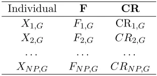
Based on these observations, we propose a new self-adaptive parameter control technique. In Gth generation, one individual corresponds to a set of control parameters (Fi,G, CRi,G), which is
shown in Table 1. Thus, the control parameters are no longer scalar quantities, but vectors. We useFG = (F1,G, F2,G, . . . , Fi,G, . . . , FNP,G) and CRG= (CR1,G, CR2,G, . . . , CRi,G, . . . , CRNP,G) in the
evolutionary process.
Table 1. Individual with control parameters.
Individual F CR
X1,G F1,G CR1,G
X2,G F2,G CR2,G
. . . . XNP,G FNP,G CRNP,G
In order to solve a specific optimization problem efficiently, the control parameter values should adapt to the problem. Our self-adaptive parameter control technique should find a set of proper control parameter values corresponding to the problem, by using the fitness values available. The SQI operator can be used to achieve this goal. Now we introduce the new self-adaptive parameter control technique in detail. Define difference scale factor intervals: Ft and Fb, Fb ⊆Ft. Define the selection intervals of the crossover probability factor: CRt and CRb,CRb⊆CRt.
In the first generation, F0 and CR0 are randomly produced in intervals Ft and CRt, respectively.
In other generations, the control parameter vectors are generated by the SQI operator. However, the produced control parameters may lie in inappropriate intervals, which may reduce the solution accuracy. In order to overcome this shortcoming, we introduce a generation interval Gt. When the generation
number is a multiple of Gt, the prior knowledge for the control parameters is used. Values in vectors FG andCRGare chosen randomly in intervals Fb andCRb, respectively. When the generation number
is not a multiple of Gt, if the produced control parameters are not in intervals Ft and CRt, we choose
the new control parameters as those corresponding to r1 in Eq. (18); Otherwise, the produced control parameters are chosen as the new ones.
It is worth to note that a selection operation for control parameters is also used for determining the appropriate control parameter values quickly. When the offspring is better than the corresponding individual, the element in the produced control parameter vectors is also selected; otherwise, it remains unchanged. By using the SQI operator with three pointsr1, r2 andr3 in the current population, values inFG are generated by Eqs. (22) and (23).
F pi,G= 0.5∗
(Fr22,G−Fr23,G)f(Xr1,G) + (Fr23,G−Fr21,G)f(Xr2,G) + (Fr21,G−Fr22,G)f(Xr3,G)
(Fr2,G−Fr3,G)f(Xr1,G) + (Fr3,G−Fr1,G)f(Xr2,G) + (Fr1,G−Fr2,G)f(Xr3,G)
(22)
F newi,G+1=
F pi,G, if F pi,G∈Ft & mod (G, Gt)= 0
Fr1,G, if F pi,G∈/Ft & mod (G, Gt)= 0
rand(Fb), if mod (G, Gt) = 0
While values in CRG are also generated by Eqs. (24) and (25).
CRpi,G= 0.5∗ (CR2
r2,G−CRr23,G)f(Xr1,G)+(CR2r3,G−CR2r1,G)f(Xr2,G)
+(CR2r1,G−CR2r2,G)f(Xr3,G)
(CRr2,G−CRr3,G)∗f(Xr1,G)+(CRr3,G−CRr1,G)
∗f(Xr2,G)+(CRr1,G−CRr2,G)∗f(Xr3,G)
(24)
CRnewi,G+1=
CRp
i,G, if CRpi,G∈CRt & mod (G, Gt)= 0
CRr1,G, if CRpi,G∈/CRt & mod (G, Gt)= 0
rand(CRb), if mod (G, Gt) = 0
i= 1,2, . . . , N P (25)
where Fnewi,G+1 and CRnewi,G+1 represent the produced control parameters for theith individual in
the G+1th generation. In order to search appropriate control parameter values quickly, the selection operation is also used for FG and CRG. Better values in vectors FG+1 and CRG+1 are selected by
Eqs. (26) and (27) respectively for the minimization problem
Fi,G+1 =
F newi,G+1, if f(Ui,G+1)< f(Xi,G+1)
Fi,G, otherwise (26)
CRi,G+1 =
CRnewi,G+1, if f(Ui,G+1)< f(Xi,G+1)
CRi,G, otherwise (27)
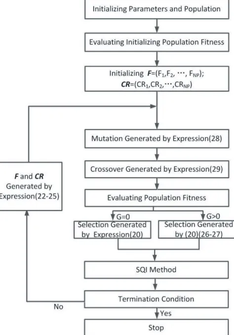
Based on the new self-adaptive parameter control technique, we propose a novel SAHDE algorithm, and its flow chart is shown in Fig. 2. And the detail procedure is presented as follows.
Step 0: Set parameters: Choose suitable N P,Ft,CRt,Fb,CRb andGt. SetG= 0.
Step 1: Initialize population: Choose randomly the initial populationX0 = (X1,0, X2,0, . . . , XNP,0) in
the feasible region.
Step 2: Evaluate the fitness values for the initial population: Calculate f(Xi,0), i= 1,2, . . . , N P.
Step 3: Produce vectors F1 and CR1: Produce Fi,1 randomly in Ft, and CRi,1 randomly in CRt,
i= 1,2, . . . , N P. Form F0= (F1,1, F2,1, . . . , FNP,1), and CR1 = (CR1,1, CR2,1, . . . , CRNP,1).
Step 4: Mutation: Calculate the mutant trial vector Vi,G+1 by using the DE mutation strategy
Vi,G+1=Xr1,G+Fi,G·(Xr2,G−Xr3,G) (28)
where indexesr1, r2, andr3 are three different random integers in range [1, N P], and also different from index i. Especially, among r1, r2, and r3 individuals in current population, r1 is the best, andr3 is the worst.
Step 5: Crossover: Calculate the offspring vectorUi,G+1 = (u1,i,G+1, u2,i,G+1, . . . , uj,i,G+1, . . . , uD,i,G+1)
by the binomial crossover operation
uj,i,G+1=
vj,i,G+1, if rand(0,1)< CRi,Gor j=rand(1, D)
xj,i,G, otherwise (29)
Step 6: Evaluate the fitness values for the offspring vector: Calculate f(Ui,G+1),i= 1,2, . . . , N P.
Step 7: Selection: Determine a new vector Xi,G+1 by using the selection operation Eq. (20).
Step 8: The SQI operation: Execute the SQI operation, as shown in the original HDE algorithm.
Step 9: Termination condition judgement: If the stopping criterion is not met, go to Step 10. Otherwise, the algorithm is terminated.
Step 10: Produce vectors FG+1 and CRG+1: First, calculate Fnewi,G+1 by using Eq. (23), and
CRnewi,G+1 by Eq. (25), i = 1,2, . . . , N P, where indexes r1, r2 and r3 are same as those in
Step 4. Then, determineFi,G+1 by Eq. (26), and CRi,G+1 by Eq. (27), i= 1,2, . . . , N P. Finally,
form FG+1 = (F1,G+1, F2,G+1, . . . , FNP,G+1), and CRG+1 = (CR1,G+1, CR2,G+1, . . . , CRNP,G+1).
SetG=G+ 1, and go toStep 4.
3.3. Numerical Experiments
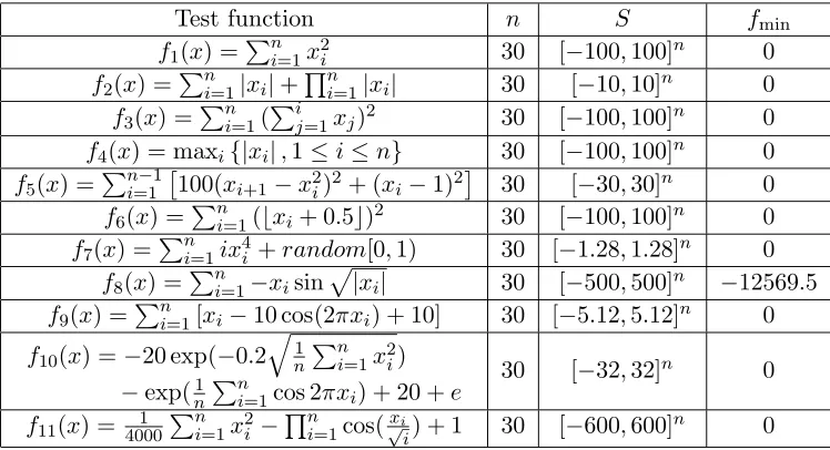
The SAHDE algorithm is tested by using 11 benchmark problems listed in Table 2. In the table, nis the dimension of the problem, S the search space, S ⊆Rn, and fmin represents the minimum value of
Table 2. Benchmark problems.
Test function n S fmin
f1(x) =
n
i=1x2i 30 [−100,100]n 0
f2(x) =
n
i=1|xi|+
n
i=1|xi| 30 [−10,10]n 0
f3(x) =
n
i=1(
i
j=1xj)2 30 [−100,100]n 0
f4(x) = maxi{|xi|,1≤i≤n} 30 [−100,100]n 0
f5(x) =
n−1
i=1
100(xi+1−x2i)2+ (xi−1)2 30 [−30,30]n 0
f6(x) =
n
i=1(xi+ 0.5 )2 30 [−100,100]n 0
f7(x) =
n
i=1ix4i +random[0,1) 30 [−1.28,1.28]n 0
f8(x) =
n
i=1−xisin
|xi| 30 [−500,500]n −12569.5
f9(x) =
n
i=1[xi−10 cos(2πxi) + 10] 30 [−5.12,5.12]n 0
f10(x) =−20 exp(−0.2
1
n
n
i=1x2i)
−exp(n1ni=1cos 2πxi) + 20 +e
30 [−32,32]n 0
f11(x) = 40001
n
i=1x2i −
n
the problem. In our experiments, the population sizeN P is set to 100. Other parameters are suggested as: Gt = 25, Ft = (0.1,2), CRt = (0.1,1), Fb = (0.4,1) and CRb = (0.5,0.95). We use the maximum
generation number Gmax as the stopping criterion IfG > Gmax, then the algorithm is terminated. For
each problem, 30 independent runs of an algorithm are tested. In order to verify the superiority of the algorithm, the results obtained by the standard DE algorithm, the jDE algorithm [18], the DESQI algorithm [22] are shown simultaneously.
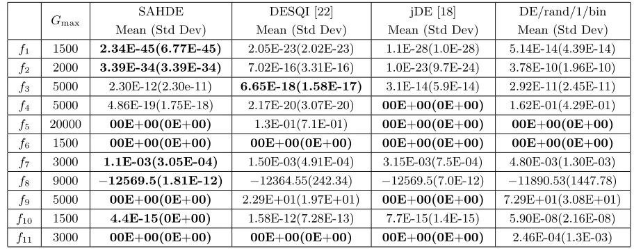
Experimental results are given in Table 3. In the table, Mean and Std Dev represent the average function value found by the algorithm and the standard deviation of the found function values for 30 independent runs, respectively. As illustrated in Table 3, for problemsf1, f2, f7, f8 andf10, the SAHDE
algorithm yields a smaller minimum objective function value. While for problemsf5, f6, f9 and f11, the
average function value found by the SAHDE algorithm is equal to that obtained by other algorithms. However, for problems f3 and f4, the average function value found by the SAHDE algorithm is a little
bit larger than that obtained by the DESQI algorithm and the jDE algorithm. Therefore, the SAHDE algorithm yields relatively accurate solutions for all the problems, and performs favorably.
Table 3. Comparison results of average function values and the standard deviations for 11 benchmark problems.
Gmax SAHDE
Mean (Std Dev)
DESQI [22] Mean (Std Dev)
jDE [18] Mean (Std Dev)
DE/rand/1/bin Mean (Std Dev)
f1 1500 2.34E-45(6.77E-45) 2.05E-23(2.02E-23) 1.1E-28(1.0E-28) 5.14E-14(4.39E-14)
f2 2000 3.39E-34(3.39E-34) 7.02E-16(3.31E-16) 1.0E-23(9.7E-24) 3.78E-10(1.96E-10)
f3 5000 2.30E-12(2.30e-11) 6.65E-18(1.58E-17) 3.1E-14(5.9E-14) 2.92E-11(2.45E-11) f4 5000 4.86E-19(1.75E-18) 2.17E-20(3.07E-20) 00E+00(0E+00) 1.62E-01(4.29E-01)
f5 20000 00E+00(0E+00) 1.3E-01(7.1E-01) 00E+00(0E+00) 00E+00(0E+00)
f6 1500 00E+00(0E+00) 00E+00(0E+00) 00E+00(0E+00) 00E+00(0E+00)
f7 3000 1.1E-03(3.05E-04) 1.50E-03(4.91E-04) 3.15E-03(7.5E-04) 4.80E-03(1.30E-03)
f8 9000 −12569.5(1.81E-12) −12364.55(242.34) −12569.5(7.0E-12) −11890.53(1447.78)
f9 5000 00E+00(0E+00) 2.29E+01(1.97E+01) 00E+00(0E+00) 7.29E+01(3.08E+01)
f10 1500 4.4E-15(0E+00) 1.58E-12(7.28E-13) 7.7E-15(1.4E-15) 5.90E-08(2.16E-08)
f11 3000 00E+00(0E+00) 00E+00(0E+00) 00E+00(0E+00) 2.46E-04(1.3E-03)
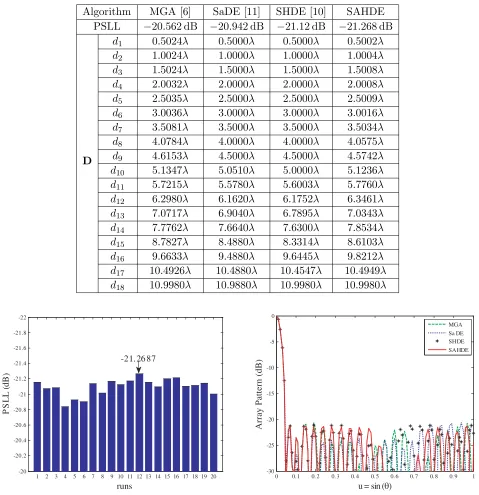
In order to prove that the SAHDE algorithm is efficient for solving array synthesis problems, the SAHDE algorithm is used to minimize the fitness function (4) under constraint of Eq. (5). To compare the algorithm with other existing algorithms, a 37-element linear aperiodic array is considered, which has been synthesized by MGA [6], SaDE [11], and SHDE [10]. The array is also symmetric and with an aperture size is equal to 21.996λ, whereλis the wavelength. That meansdM = 10.998λ. Here, dmin is
set to 0.5λ.
For the SAHDE algorithm, we choose N P = 80. Other parameters are chosen as suggested. The termination condition is that the maximum number of function evaluations reaches 40000. The optimal PSLLs and element positions are illustrated in Table 4. Compared with other algorithms, the SAHDE algorithm yields−21.268 dB PSLL, which is better than−20.562 dB by MGA [6], −20.942 dB by SaDE [11] and −21.12 dB by SHDE [10]. As shown in Fig. 3, the PSLLs obtained by the SAHDE algorithm for the array in 20 independent runs are stable. Comparison of the radiation patterns obtained by four algorithms for the array is also shown in Fig. 4. Simulated results indicate that the SAHDE algorithm yields better results than other existing algorithms in the same conditions. Results demonstrate the SAHDE algorithm is efficient for solving the array synthesis problem.
Table 4. PSLLs and element positions for the 37-element sparse linear array.
Algorithm MGA [6] SaDE [11] SHDE [10] SAHDE PSLL −20.562 dB −20.942 dB −21.12 dB −21.268 dB
D
d1 0.5024λ 0.5000λ 0.5000λ 0.5002λ
d2 1.0024λ 1.0000λ 1.0000λ 1.0004λ
d3 1.5024λ 1.5000λ 1.5000λ 1.5008λ
d4 2.0032λ 2.0000λ 2.0000λ 2.0008λ
d5 2.5035λ 2.5000λ 2.5000λ 2.5009λ
d6 3.0036λ 3.0000λ 3.0000λ 3.0016λ
d7 3.5081λ 3.5000λ 3.5000λ 3.5034λ
d8 4.0784λ 4.0000λ 4.0000λ 4.0575λ
d9 4.6153λ 4.5000λ 4.5000λ 4.5742λ
d10 5.1347λ 5.0510λ 5.0000λ 5.1236λ
d11 5.7215λ 5.5780λ 5.6003λ 5.7760λ
d12 6.2980λ 6.1620λ 6.1752λ 6.3461λ
d13 7.0717λ 6.9040λ 6.7895λ 7.0343λ
d14 7.7762λ 7.6640λ 7.6300λ 7.8534λ
d15 8.7827λ 8.4880λ 8.3314λ 8.6103λ
d16 9.6633λ 9.4880λ 9.6445λ 9.8212λ
d17 10.4926λ 10.4880λ 10.4547λ 10.4949λ
d18 10.9980λ 10.9880λ 10.9980λ 10.9980λ
1 2 3 4 5 6 7 8 9 10 11 12 13 14 15 16 17 18 19 20 -22
-21.8
-21.6
-21.4
-21.2
-21
-20.8
-20.6
-20.4
-20.2
-20
runs
P
S
LL (
d
B
)
-21. 26 87
Figure 3. PSLLs obtained by the SAHDE algo-rithm for the 37-element array in 20 independent runs.
0 0. 1 0. 2 0. 3 0. 4 0. 5 0. 6 0. 7 0. 8 0. 9 1
-30 -25 -20 -15 -10 -5 0
u = sin (θ)
Array Pattern (dB)
MGA Sa DE SHDE SAHDE
Figure 4. Comparison of the radiation patterns obtained by four algorithms for the 37-element array.
4. WORST-CASE TOLERANCE SYNTHESIS OF LOW-SIDELOBE SPARSE LINEAR ARRAYS BY USING THE SAHDE ALGORITHM
computational burden greatly. In [14], Jiao et al. chose the vertices of the tolerance region as the sample point candidates for calculating the worst-case PSLLs of the linear arrays. However, Problem (16) is a non-convex problem, and the worst cases may not appear in the vertexes of the tolerance region. In order to solve this problem, we present a fast way for calculating the fitness function (17).
Although Problem (16) is a non-convex problem, the points around boundary of the tolerance region in Eq. (11) have greater contribution to the worst-case PSLLs of the sparse linear array, while the points far from its boundary have very little contribution. In order to calculate the fitness function (17) efficiently, we choose some sample points around boundary of the tolerance region in Eq. (11) randomly.
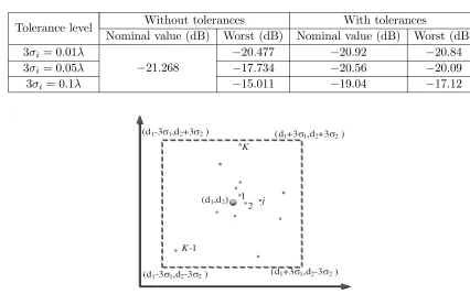
Since it is difficult to depict the multidimensional problem, the 2-dimensional problem is taken as an example to illustrate the sampling way. Fig. 5 shows schematic diagram of the sampling way. In the figure, (d1,d2) denotes the nominal element position vector, and the dash-line box represents boundary
of the tolerance region in Eq. (11). The sample points are chosen randomly around boundary of the region based on the Gaussian distribution. Define the Chebyshev distance between the sample point and the nominal element position vector as
dchj = max
d1+dcj1
−d1,
d2+dcj2
−d2
= maxdcj1,dcj2
(30)
The greater the Chebyshev distance is, the closer the sample point approaches the boundary. In the tolerance region, we recommend to choose some sample points with greater Chebyshev distances instead of choosing all the points. Only these sample points are used to calculate the fitness function (17). The detail procedure for calculating the fitness function is presented as follows.
Step 0: Set parameters: Set the fixed standard deviation σi, the tolerance region for every element position (−3σi,3σi), i = −M,−(M −1), . . . ,0, . . . , M −1, M, the total sample point number J, and the used sample point numberN S (N S < J) in Eq. (17).
Step 1: Produce error vectors: ProduceJDcvectors in the tolerance region (11) based on Eq. (10).
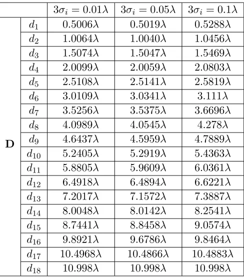
Table 5. Optimal element positions for the 37-element sparse linear array.
3σi = 0.01λ 3σi = 0.05λ 3σi = 0.1λ
D
d1 0.5006λ 0.5019λ 0.5288λ
d2 1.0064λ 1.0040λ 1.0456λ
d3 1.5074λ 1.5047λ 1.5469λ
d4 2.0099λ 2.0059λ 2.0803λ
d5 2.5108λ 2.5141λ 2.5819λ
d6 3.0109λ 3.0341λ 3.111λ
d7 3.5256λ 3.5375λ 3.6696λ
d8 4.0989λ 4.0545λ 4.278λ
d9 4.6437λ 4.5959λ 4.7889λ
d10 5.2405λ 5.2919λ 5.4363λ
d11 5.8805λ 5.9609λ 6.0361λ
d12 6.4918λ 6.4894λ 6.6221λ
d13 7.2017λ 7.1572λ 7.3887λ
d14 8.0048λ 8.0142λ 8.2541λ
d15 8.7441λ 8.8458λ 9.0574λ
d16 9.8921λ 9.6786λ 9.8464λ
d17 10.4968λ 10.4866λ 10.4883λ
Step 2: Calculate the Chebyshev distance: Calculate the Chebyshev distance between every Dc and the nominal element position vector by Eq. (30), sort the distances in the descending order, and choose N S sample points with larger Chebyshev distances.
Step 3: Evaluate the fitness function: TheN S sample points are used to calculate the fitness function value by Eq. (17).
Parameters J and N S are set as 50000 and 2500, respectively. The SAHDE algorithm is used to solve Problem (16). For its control parameters and the termination condition, refer to Section 3.
When the tolerance regions are fixed to three levels 3σi = 0.01λ, 0.05λ, 0.1λ, the optimal element
positions are given in Table 5, and the optimal PSLLs are shown in Table 6. The worst PSLLs are
Table 6. Optimal PSLLs for the 37-element sparse linear array.
Tolerance level Without tolerances With tolerances
Nominal value (dB) Worst (dB) Nominal value (dB) Worst (dB) 3σi = 0.01λ
−21.268
−20.477 −20.92 −20.84
3σi = 0.05λ −17.734 −20.56 −20.09
3σi = 0.1λ −15.011 −19.04 −17.12
(d1,d2) 1
2 j
K-1
K
(d1-3σ1,d2-3σ2) (d1+3σ1,d2-3σ2)
(d1+3σ1,d2+3σ2)
(d1-3σ1,d2+3σ2)
Figure 5. Schematic diagram of the sampling way.
(a) (b)
-1 -0.8 -0.6 -0.4 -0.2 0 0.2 0.4 0.6 0.8 1 -80
-70 -60 -50
-40 -30 -20 -10 0
Array Pattern (dB)
Nominal Worst-case
-1 -0.8 -0.6 -0.4 -0.2 0 0.2 0.4 0.6 0.8 1 -80
-70 -60 -50 -40 -30 -20 -10 0
Nominal Worst-case
Array Pattern (dB)
(c)
-1 -0.8 -0.6 -0.4 -0.2 0 0.2 0.4 0.6 0.8 1 -60
-50 -40 -30 -20 -10 0
Nominal Worst-case
Array Pattern (dB)
u = sin (θ)
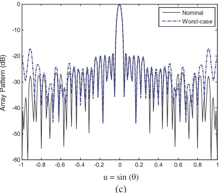
Figure 6. Comparison of the radiation patterns for the 37-element sparse linear array with three fixed position tolerance levels. (a) 3σi = 0.01λ. (b) 3σi= 0.05λ. (c) 3σi= 0.1λ.
−20.84 dB,−20.09 dB and−17.12 dB, and the nominal PSLLs are−20.92 dB,−20.56 dB and−19.04 dB. As comparison, without considering the element position errors, the nominal PSLL is −21.268 dB, as shown in Table 4. Analysis results show that the worst PSLLs are −20.477 dB, −17.734 dB and −15.011 dB, corresponding to three tolerance levels. Although the nominal PSLLs−20.92 dB,−20.56 dB and −19.04 dB obtained by the tolerance optimization are higher than−21.268 dB without considering the errors, the worst-case PSLLs are improved from−20.477 dB to−20.84 dB,−17.734 dB to−20.09 dB and −15.011 dB to −17.12 dB, as shown in Table 6. Comparison of the radiation patterns considering the errors are also shown in Fig. 6. The compared results show that the worst-case peak sidelobe levels for the sparse linear arrays are improved evidently.
5. CONCLUSION
In this paper, a worst-case tolerance synthesis for low-sidelobe sparse linear arrays with random position errors has been studied. First, the worst-case tolerance synthesis model considering random position errors is established. Through the random sampling, the random optimization problem is converted to a deterministic optimization problem. In order to solve the problem, a novel self-adaptive hybrid differential evolution algorithm is proposed then, in which a novel self-adaptive parameter control technique is adopted. The control parameters have been produced by the simplified quadratic interpolation operator, and the connections between control parameters and fitness values available are established. In order to determine the appropriate control parameter values quickly, a selection operation for control parameters is also used. 11 benchmark problems have been used for verifying the effectiveness of the algorithm. Moreover, a sparse linear array is synthesized by using the SAHDE algorithm. Simulated results demonstrate that the SAHDE algorithm is efficient not only for global optimization problems, but also for synthesizing low sidelobe sparse antenna arrays. Finally, the worst-case tolerance synthesis problems with three fixed position tolerance levels are solved by the SAHDE algorithm. Simulated results illustrate that the worst PSLLs have been improved evidently. The SAHDE algorithm can also be used to solve the worst-case tolerance synthesis for other antenna arrays.
REFERENCES
2. Skolnik, M. I., G. Nemhauser, and J. W. Sherman, “Dynamic programming applied to unequally spaced arrays,” IEEE Trans. Antennas Propag., Vol. 12, No. 1, 35–43, Jan. 1964.
3. Kumar, B. P. and G. R. Branner, “Design of unequally for performance improvement,” IEEE Trans. Antennas Propag., Vol. 47, No. 3, 511–523, Mar. 1999.
4. Haupt, R. L, “Unit circle representation of aperiodic arrays,” IEEE Trans. Antennas Propag., Vol. 43, No. 10, 1152–1155, Oct. 1995.
5. Haupt, R. L., “Thinned arrays using genetic algorithms,”IEEE Trans. Antennas Propag., Vol. 42, No. 7, 993–999, Jul. 1994.
6. Cheng, K. S., Z. S. He, and C. L. Han, “A modified real GA for the sparse linear array synthesis with multiple constraints,”IEEE Trans. Antennas Propag., Vol. 54, No. 7, 2169–2173, Jul. 2006. 7. Khodier, M. M. and C. G. Christodoulou, “Linear array geometry synthesis with minimum sidelobe
level and null control using particle swarm optimization,” IEEE Trans. Antennas Propag., Vol. 53, No. 8, 2674–2679, Aug. 2005.
8. Rocca, P., G. Oliveri, and A. Massa, “Differential evolution as applied to electromagnetics,” IEEE Antennas and Propagation Magazine, Vol. 53, No. 1, 38–49, 2011.
9. Cen, L., Z. L. Yu, and W. Ser, “Linear aperiodic array synthesis using an improved genetic algorithm,”IEEE Trans. Antennas Propag., Vol. 60, No. 2, 895–902, Feb. 2012.
10. Zhang, L., Y. C. Jiao, B. Chen, and F. S. Zhang, “Synthesis of linear aperiodic arrays using a self-adaptive hybrid differential evolution algorithm,” IET Microwaves, Antennas & Propag., Vol. 5, No. 12, 1524–1528, Dec. 2011.
11. Goudos, S. K., K. Siakavara, T. Samaras, E. E. Vafiadis, and J. N. Sahalos, “Sparse linear array synthesis with multiple constraints using differential evolution with strategy adaptation,” IEEE Antennas and Wire. Propag. Lett., Vol. 10, 670–673, 2011.
12. Schjaer-Jacobsen, H. and K. Madsen, “Algorithms for worst case tolerance optimization,” IEEE Trans. Circuits &Systems, Vol. 26, No. 9, 775–783, Sep. 1979.
13. Schjaer-Jacobsen, H., “Worst-case tolerance optimization of antenna system,” IEEE Trans. Antennas Propag., Vol. 28, No. 2, 247–250, Mar. 1980.
14. Jiao, Y. C., Y. H. Qi, and L.-Y. Zhang, “Tolerance optimization design for low sidelobe linear arrays,” IEEE Antennas and Propagation Society International Symposium, 736–739, 1993. 15. Anselmi, N., L. Manica, P. Rocca, and A. Massa, “Tolerance analysis of antenna arrays through
interval arithmetic,” IEEE Trans. Antennas Propag., Vol. 61, No. 11, 5496–5507, Nov. 2013. 16. Krischuk, V., G. Shilo, and B. Artyushenko, “Tolerable linear antenna array design with genetic
algorithm,”9th International Conference onthe Experience of Designing and Applications of CAD Systems in Microelectronics, 167–169, 2007.
17. Qin, A. K. and P. N. Suganthan, “Self-adaptive differential evolution algorithm for numerical optimization,” 2005 IEEE Congress on Evolutionary Computation, Vol. 2, 1785–1791, 2005. 18. Brest, J., S. Greiner, B. Boskovic, and V. Zumer, “Self-adapting control parameters in differential
evolution: A comparative study on numerical benchmark problems,”IEEE Trans. on Evolutionary Computation, Vol. 10, No. 6, 646–657, Jun. 2006.
19. Ali, M. M., A. Torn, and S. Vitanen, “A numerical comparison of some modified controlled random search algorithms,”J. Global Optim., Vol. 11, 377–385, 1997.
20. Jiao, Y. C., C. Dang, Y. Leung, and Y. Hao, “A modification to the new version of the Price’s algorithm for continuous global optimization problems,” J. Global Optim., Vol. 36, 609–626, 2006. 21. Li, H., Y. C. Jiao, and Y. P. Wang, “Integrating the simplified interpolation into the genetic algorithm for constrained optimization problems,” Computational Intelligence and Security, 247– 254, Lecture Notes in Artificial Intelligence 3801, Springer-Verlag, Berlin, 2005.
22. Zhang, L., Y. C. Jiao, H. Li, and F. S. Zhang, “Antenna optimization by hybrid differential evolution,”Int. J. RF and Microwave Comput. — Aided Eng., Vol. 20, 51–55, 2010.
24. Azaro, R., G. Boato, M. Donelli, et al., “Design of a prefractal monopolar antenna for 3.4–3.6 GHz Wi-Max band portable devices,” IEEE Antennas and Wire. Propag. Lett., Vol. 5, 116–119, 2007. 25. Carlo, F., D. Massimo, and G. F. Walsh, “Particle-swarm optimization of broadband nanoplasmonic
arrays,” Optics Letters, Vol. 35, No. 2, 133–135, 2010.
26. Azaro, R., F. G. B. De Natale, M. Donelli, et al. “Optimized design of a multifunction/multiband antenna for automotive rescue systems,” IEEE Trans. Antennas Propag., Vol. 54, No. 2, 392–400, Feb. 2006.
27. Donelli, M., I. J. Craddock, D. Gibbins, and M. Sarafianou, “A three-dimensional time domain microwave imaging method for breast cancer detection based on an evolutionary algorithm,” Progress In Electromagnetics Research M, Vol. 18, 179–195, 2011.
28. Oliveri, G., M. Donelli, and A. Massa, “Linear array thinning exploiting almost difference sets,” IEEE Trans. Antennas Propag., Vol. 57, No. 12, 3800–3812, Dec. 2009.
29. Oliveri, G., M. Donelli, and A. Massa, “ADS-based guidelines for thinned planar arrays,” IEEE Trans. Antennas Propag., Vol. 58, No. 6, 1935–1948, Jun. 2010.
30. Oliveri, G. and A. Massa, “Bayesian compressive sampling for pattern synthesis with maximally sparse non-uniform linear arrays,” IEEE Trans. Antennas Propag., Vol. 59, No. 2, 467–481, Feb. 2011.
31. Viani, F., G. Oliveri, and A. Massa, “Compressive sensing pattern matching techniques for synthesizing planar sparse arrays,” IEEE Trans. Antennas Propag., Vol. 61, No. 9, 4577–4587, Sep. 2013.
32. Poli, L., P. Rocca, N. Anselmi, and A. Massa, “Dealing with uncertainties on phase weighting of linear antenna arrays by means of interval-based tolerance analysis,” IEEE Trans. Antennas Propag., Vol. 63, No. 7, 3229–3234, Jul. 2015.
33. Rocca, P., N. Anselmi, and A. Massa, “Optimal synthesis of robust array configurations exploiting interval analysis and convex optimization,” IEEE Trans. Antennas Propag., Vol. 62, No. 7, 3603– 3612, Jul. 2014.