Shielding of a Perfectly Conducting Circular Disk: Exact and Static
Analytical Solution
Giampiero Lovat1, *, Paolo Burghignoli2, Rodolfo Araneo1, Salvatore Celozzi1, Amedeo Andreotti3, Dario Assante4, and Luigi Verolino3
Abstract—The problem of the shielding evaluation of an infinitesimally thin perfectly conducting circular disk against a vertical magnetic dipole is here addressed. The problem is reduced to a set of dual integral equations and solved in an exact form through the application of the Galerkin method in the Hankel transform domain. It is shown that a second-kind Fredholm infinite matrix-operator equation can be obtained by selecting a complete set of orthogonal eigenfunctions of the static part of the integral operator as expansion basis. A static solution is finally extracted in a closed form which is shown to be accurate up to remarkably high frequencies.
1. INTRODUCTION
The interaction of electromagnetic waves with a circular metal disk constitutes a classical diffraction problem that, along with its Babinet-complementary problem of diffraction by a circular hole in an infinite metal plate, has received considerable interest in the literature of the last decades (see, e.g., [1– 16] and references therein). Such a canonical configuration is in fact of interest for scattering (e.g., radar cross-section evaluation), antennas, as well as electromagnetic-shielding problems.
In this paper we consider the incidence of spherical waves produced by a point source placed at a finite distance from a circular perfectly-conducting (PEC) disk, namely a Vertical Magnetic Dipole (VMD) placed along the axis of azimuthal symmetry of the structure. This canonical source constitutes a valid representation for a practical small electric-loop radiator parallel to the disk and co-axial with it.
The formulation of the problem is first presented in Section 2, and operating in the Hankel transform domain, a set of dual integral equations (whose unknown is the surface current density induced on the PEC disk) is derived. An exact numerical solution, valid in any frequency range, is obtained in Section 3 through the application of Galerkin’s Method of Moments choosing a set of orthogonal eigenfunctions of the static part of the involved integral operator as expansion functions for the surface current induced on the disk. It is shown that such functions allow for a rapidly convergent representation of the unknown since they reconstruct the physical behavior of the surface current density both at the center and at the edges of the disk. The rapidly converging properties of such a numerical solution are also improved by a suitable series representation of the elements of the impedance matrix. One very interesting result of the present work (presented in Section 4) is that, thanks to different integral identities, the static-limit solution can be extracted in a closed form, and such a closed form is shown to be accurate up to remarkably high frequencies, depending on the involved geometric parameters of the problem.
Received 29 May 2019, Accepted 10 August 2019, Scheduled 5 September 2019
* Corresponding author: Giampiero Lovat ([email protected]).
1 Department of Astronautical, Electrical, and Energetic Engineering, Sapienza University of Rome, Italy. 2 Department of
It is important to point out, as rigorously shown in Section 5, that the proposed solution scheme fits into the more general method of analytical regularization already proposed with success in the literature [9, 12, 15, 16]. Finally, in Section 6, the conclusions of the present investigation are drawn.
2. FORMULATION OF THE PROBLEM
The configuration under analysis consists of an infinitesimally thin, perfectly conducting (PEC) circular disk of radiusaplaced on the planez= 0 of a cylindrical coordinate system (ρ, φ, z) with center at the origin and a vertical magnetic dipole (VMD) with magnetic dipole moment mplaced along the z axis at a height z=h (see Fig. 1) and coaxial with it. The vertical magnetic dipole can effectively model a small current loop parallel to the plane z= 0 and coaxial with the disk. The electromagnetic problem is axially symmetric so that all the fields depend only on ρ and z. Time-harmonic sources and fields are assumed with an implicit ejωt dependence.
VMD
O
y
z
ρ
φ
z
h
0
a
x
Figure 1. Configuration under analysis: a vertical magnetic dipole (VMD) radiates in the presence of a circular perfectly conducting (PEC) disk with radius a and of negligible thickness. The VMD is axially symmetric with respect to the disk and placed at a distanceh from it.
2.1. Electric Field of a Current Loop
We first consider an electric current loop of radius ρ0 placed over the planez=z0. Therefore
J(ρ, z) =Jφ(ρ, z)uφ=P0δ
(ρ−ρ0)
ρ δ(z−z0)uφ (1) whereP0is a suitable coefficient. The vector potentialAhas only the componentAφwhich must satisfy the Helmholtz equation, which in cylindrical coordinates reads
∂2Aφ ∂z2 +
1 ρ
∂ ∂ρ
ρ∂Aφ
∂ρ
−Aφ
ρ2 +k0Aφ=−μ0Jφ (2) wherek0 is the free-space wavenumber. By introducing the Hankel transform of order 1 defined as [17]
˜
F(λ) =H1{F(ρ)}=
∞
0
ρF(ρ)J1(λρ)dρ
F(ρ) =H1−1{F˜(λ)}=
∞
0
λF˜(λ)J1(λρ)dλ
(3)
whereJ1(·) is the first-kind Bessel function of order 1, we have [17]
∂2A˜φ ∂z2 −λ
2A˜
By letting kz =k20−λ2 =−j
λ2−k2
0 and by Hankel-transforming the current (1) (which samples the Bessel functionJ1 inρ0) we obtain
∂2A˜φ ∂z2 +k
2
zA˜φ=−μ0P0J1(λρ0)δ(z−z0) (5)
whose solution is
˜
Aφ(λ, z) =μ0P0J1(λρ0)e
−jkz|z−z0|
2jkz (6)
By Hankel inverse-transforming, we thus have
Aφ(ρ, z) = μ2j0P0
∞
0
e−jkz|z−z0|
kz J1(λρ0)J1(λρ)λdλ (7) Since ∇ ·A= 0, it follows that E=−jωA and therefore
Eφ(ρ, z) =−k0ζ20P0
∞
0
e−jkz|z−z0|
kz J1(λρ0)J1(λρ)λdλ (8) whereζ0 is the free-space characteristic impedance.
2.2. Electric Field of a Current Disk
By considering a disk of radius a placed in z0 = 0, with a current density J(ρ, z) = JSφ(ρ)δ(z)uφ, by integrating (8) withP0=ρ0JSφ(ρ0), we obtain
Eφ(ρ, z) =−k02ζ0
a
0
ρ0JSφ(ρ0)
∞
0
e−jkz|z|
kz J1(λρ0)J1(λρ)λdλdρ0 (9) and rearranging
Eφ(ρ, z) =−k02ζ0
∞
0
a
0
ρ0JSφ(ρ0)J1(λρ0)dρ0
e−jkz|z|
kz J1(λρ)λdλ (10) By introducing the Hankel transform of the current density, we have
Eφ(ρ, z) =−k02ζ0
∞
0 ˜ JSφ(λ)e
−jkz|z|
kz J1(λρ)λdλ (11)
2.3. Electric Field of a Magnetic Dipole
By indicating the moment of a current loop placed inz0 =hwith|m|=Iπρ20, the relevant electric field is expressed as
Eφinc(ρ, z) =−k0ζ0|m| 2πρ0
∞
0
e−jkz|z−h|
kz J1(λρ0)J1(λρ)λdλ (12) In the limit ρ0 →0 (sinceJ1(x)x/2), we obtain
Eφinc(ρ, z) =−k0ζ0|m| 4π
∞
0
e−jkz|z−h|
kz J1(λρ)λ 2d
λ (13)
2.4. Boundary Condition
Since we assume a perfectly conducting disk, the tangential component (i.e., theφ component) of the total electric field E vanishes atz= 0 forρ < a, i.e.,
Escatφ (ρ, z= 0) +Eφinc(ρ, z = 0) = 0 (14) By using Eqs. (11) and (13) for z= 0 andρ < a, we thus have
−k0ζ0
∞
0 1
2kzJ1(λρ) ˜JSφ(λ)λdλ−k0ζ0|m|
∞
0
e−jkzh
4πkz J1(λρ)λ 2d
i.e., ∞
0 1
kzJ1(λρ) ˜JSφ(λ)λdλ+ |m|
2π
∞
0
e−jkzh
kz J1(λρ)λ
2dλ= 0 (16)
This equation and the condition for which the current density vanishes forρ > aconstitute a system of dual integral equations. By rearranging we obtain
∞
0 1 kz
˜
JSΦ(λ) + | m|λ
2π e −jkzh
J1(λρ)λdλ= 0, ρ < a
∞
0 ˜
JSφ(λ)J1(λρ)λdλ= 0, ρ > a
(17)
3. GALERKIN METHOD-OF-MOMENTS SOLUTION
The unknown current density JSφ can be expanded through a set of basis functions bn(ρ) whose transform ˜bn(λ) should automatically satisfy the second in Eq. (17) and correctly reproduce the singular behavior of the current in ρ=a. Therefore we must have
∞
0
˜bn(λ)J1(λρ)λdλ= 0 (18)
forρ > aand
bn(ρ) =
∞
0
˜bn(λ)J1(λρ)λdλ∝ 1
a2−ρ2 (19)
forρ < a. Moreover, in the origin the value ofbn has to be finite or, better, identically zero. A possible set of basis functions is therefore provided by the following integral identity [18]
+∞
0
J2m−1+k(λ a)
(λ a)k J1(λρ)λdλ= ⎧ ⎪ ⎨ ⎪ ⎩
0 ρ > a
B(m, k) a2k+1 ρ
a2−ρ2k−1Pm(1−,k1−1)
1−2ρ 2
a2
ρ < a (20)
where
B(m, k) = (m−1)!
2k−1Γ (m+k−1) (21)
and Pn(α,β)(·) are the Jacobi polynomials of ordernand Γ (·) is the Gamma function. Therefore
H−1 1
J2m−1+k(λ a) (λ a)k
= B(m, k) a2k+1 ρ
a2−ρ2k−1Pm(1−,k1−1)
1− 2ρ 2
a2
u−1(a−ρ) (22)
We can thus adopt the following set of basis functions:
bn(ρ) = ⎧ ⎪ ⎨ ⎪ ⎩
0 ρ > a
√
2(n−1)! Γ (n−1/2)
ρ aa2−ρ2P
(1,−1/2) n−1
1− 2ρ
2
a2
, n= 1,2, . . . ρ < a (23)
which satisfy all the required conditions and whose Hankel transforms are
˜bn(λ) =
a
λJ2n−1/2(λ a) (24) We can thus express
JSφ(ρ) = +∞
n=1
and
˜
JSφ(λ) = +∞
n=1
in˜bn(λ) (26)
By using the basis-function expansion and projecting on the generic basis functionbm(ρ) we obtain
a
0
ρbm(ρ)
∞ 0 1 kz ∞ n=1
in˜bn(λ)J1(λρ)λdλdρ=−
a
0
ρbm(ρ)
∞
0
|m|λ 2πkze
−jkzh
J1(λρ)λdλdρ (27)
By truncating the expansion of the current density toN basis functions we have N n=1 in ∞ 0 ˜
bm(λ) 1 kz
˜
bn(λ)λdλ=−
∞
0 ˜
bm(λ)|m|λ 2
2πkz e
−jkzhdλ, m= 1, . . . , N (28)
i.e,
N
n=1
inZmn=Vm, m= 1, . . . , N (29)
where
Zmn=
∞
0 ˜
bm(λ) ˜bn(λ)
kz λdλ (30)
and
Vm=−
∞
0 ˜
bm(λ)|m|λ 2
2πkz e
−jkzhdλ (31)
The solution of the algebraic system in Eq. (29) furnishes the coefficients in, and the current density JSφ is recovered through Eq. (25).
In particular, from Eqs. (30) and (24) we have
Zmn=
∞
0
a
λJ2m−1/2(λ a)
a
λJ2n−1/2(λ a) 1
k02−λ2
λdλ=a
∞
0
J2m−1/2(λ a)J2n−1/2(λ a) k02−λ2
dλ (32)
In general, the improper integrals in Eq. (32) are highly oscillating and slowly decaying. However, as shown in [16], they can be transformed in
∞
0
J2m−1/2(λ a)J2n−1/2(λ a)
k20−λ2
dλ= π/2
0
J2m−1/2(k0asint)H2(2)n−1/2(k0asint)dt (33)
ifm≥n, whereHν(2)(·) is the second-kind Hankel function of order ν, and
∞
0
J2m−1/2(λ a)J2n−1/2(λ a)
k20−λ2
dλ= π/2
0
J2n−1/2(k0asint)H2(2)m−1/2(k0asint)dt (34)
ifn > mso that
Zmn=a π/2
0
J2 max{m,n}−1/2(k0asint)H2 min(2) {m,n}−1/2(k0asint)dt (35)
It can immediately be seen that the matrix [Zmn] is symmetric, i.e., Zmn=Znm.
Alternatively, the integrals in Eq. (32) can be evaluated through a rapidly converging series as [19]
∞
0
J2m−1/2(λ a)J2n−1/2(λ a)
k2 0−λ2
dλ= (−1) p
2k0a +∞
l=1
−l+ 1
2 p −l 2 q
(jk0a)l
Γ
l+ 1 2 +p
Γ
l 2 +q
Γ
l+ 1
2
wherep=n−m,q=n+m and (x)y is the Pochhammer symbol defined as
(x)y = Γ (x+y)
Γ (x) (37)
so that
Zmn = j(−1) n−ma
2 +∞ l=1 Γ l 2 Γ −l+ 1
2 +n−m
Γ
−l
2+n+m
(jk0a)l−1
Γ
l+ 1 2
Γ
−l+ 1
2
Γ
−l+ 2 2
Γ
l−1
2 +n−m
Γ
l
2 +n+m
(38)
As concerns the known term, we have
Vm=−
∞
0
a
λJ2m−1/2(λ a) |m|λ2
2πkz e
−jkzhdλ=−|m| √
a 2π
∞
0
J2m−1/2(λ a)λ3/2
e−j√k20−λ2h
k02−λ2
dλ (39)
3.1. Electric and Magnetic Fields
Once thein coefficients are known (and thus the currentJSφ as well), the radiated electric field is given by
Eφ(ρ, z) =Eφinc(ρ, z) +Eφscat(ρ, z) (40) where
Eφinc(ρ, z) =−k0ζ0|m| 4π
∞
0
e−jkz|z−h|
kz J1(λρ)λ
2dλ (41)
and
Eφscat(ρ, z) =−k0ζ0 2 N n=1 in ∞ 0 ˜ bn(λ)e
−jkz|z|
kz J1(λρ)λdλ (42) The magnetic field is instead given by
H(ρ, z) =−∇ ×E jk0ζ0
= j k0ζ0
−∂Eφ
∂z uρ+ 1 ρ
∂
∂ρ(ρEφ)uz
(43)
and therefore
Hρinc(ρ, z) = |m| 4π
∞
0
e−jkz|z−h|J
1(λρ)λ2dλ (44)
Hzinc(ρ, z) = −j|m| 4π
∞
0
e−jkz|z−h|
kz J0(λρ)λ 3d
λ (45)
and
Hρscat(ρ, z) = 1 2 N n=1 in ∞ 0 ˜
bn(λ)e−jkz|z|J1(λρ)λdλ (46)
Hzscat(ρ, z) = −j 2 N n=1 in ∞ 0
˜bn(λ)e−jkz|z| kz λ
2
J0(λρ) dλ (47)
We thus have
Eφscat(ρ, z) = −k0ζ0 √ a 2 N n=1 in ∞ 0
J2n−1/2(λ a)J1(λρ) √
λe
−j√k20−λ2|z|
k2 0 −λ2
dλ (48)
Hρscat(ρ, z) = √ a 2 N n=1 in ∞ 0
J2n−1/2(λ a)J1(λρ) √
λe−j √
k2
0−λ2|z|dλ (49)
Hzscat(ρ, z) = −j √ a 2 N n=1 in ∞ 0
J2n−1/2(λ a)J0(λρ)λ3/2e
−j√k20−λ2|z|
k2 0 −λ2
4. STATIC SOLUTION
It is interesting to note that in the static limit (i.e., k0 →0) the elements Zmn in Eq. (32) become
Zmn= ja
∞
0
J2m−1/2(λ a)J2n−1/2(λ a)
λ dλ (51)
Such an integral can be evaluated in a closed form using the identity [20, 6.574]
∞
0
Jν(αt)Jμ(αt)t−λdt=
αλ−1Γ (λ) Γ
ν+μ−λ+ 1 2
2λΓ
−
ν+μ+λ+ 1 2
Γ
ν+μ+λ+ 1 2
Γ
ν−μ+λ+ 1 2
(52)
valid for ν+μ+ 1> λ > 0 and α >0. In fact, by letting ν = 2m−1/2, μ= 2n−1/2, α =a,t=λ, and λ= 1, we have
Zmn=
jaΓ
m+n−1 2
2Γ (n−m+ 1) Γ
m+n+1 2
Γ (m−n+ 1)
(53)
On the other hand, the integral in Eq. (51) is the product of two orthogonal functions: therefore, as can be verified by observing the denominator in Eq. (53) (which is always infinite except for the case m=n), we have Zmn = 0 form=nand
Znn= ja 2
Γ
2n−1 2
Γ
2n+1 2
(54)
It is worth noting that the result in Eq. (54) can also be obtained from Eq. (38), by observing that in the static limit only the term l= 1 of the series is different from zero. By considering the property of the Gamma function for which
Γ(z+ 1) =zΓ(z) (55)
Eq. (54) can also be expressed in a simpler way as
Znn= ja
(4n−1) (56)
Concerning the known term, from Eq. (39), in the static limit we have
Vm =−j|m| √
a 2π
∞
0
J2m−1/2(λ a) √
λe−λhdλ (57)
Also the latter integral can be expressed in a closed form by using the identity [20, 6.621]
∞
0
e−αxJν(βx)xμ−1dx=α2+β2−μ/2Γ(ν+μ)Pμ−−ν1
αα2+β2−1/2
(58)
valid for α >0, β > 0, ν+μ >0, and where Pμν(·) are the associated Legendre functions of the first kind. In fact, by letting α=h,ν = 2m−1/2, β=a, and μ= 3/2, we thus have
Vm=−j|m| 2π
(2m)!√a
(a2+h2)3/4P
−2m+1/2 1/2
ha2+h2−1/2
(59)
By collecting all the results, we have N
n=1
where
Zmn= ⎧ ⎨ ⎩
0 m=n
ja
(4n−1) m=n
(61)
and
Vm=−j|2m| π
(2m)!√a
(a2+h2)3/4P
−2m+1/2 1/2
h √
a2+h2
(62)
Since the system is diagonal, we immediately obtain
in=−|m| 2π
(2n)! (4n−1) √
a(a2+h2)3/4P
−2n+1/2 1/2
h √
a2+h2
(63)
so that, from Eq. (25), in the static limit we have
JSφ(ρ) =− |m| +∞
n=1
(2n)!(n−1)! (4n−1) √
2πΓ (n−1/2)a3/2(a2+h2)3/4P
−2n+1/2 1/2
h √
a2+h2
· ρ a2−ρ2P
(1,−1/2) n−1
1−2ρ
2
a2
(64)
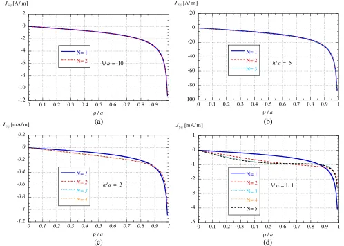
The excellent convergence properties of the basis functions and the behavior of the surface current as a function of the ratio r/afor different values ofh/a are reported in Fig. 2.
It is also interesting to observe the variation of the surface current as a function of the radiusafor a fixed value ofh= 30 cm, as shown in Fig. 3.
From Eqs. (41), (44), and (48)–(50), in the static limit we also haveEφ= 0 and
Hρinc(ρ, z) = |m| 4π
∞
0
e−λ|z−h|J1(λρ)λ2dλ (65)
Hzinc(ρ, z) = |m| 4π
∞
0
e−λ|z−h|J0(λρ)λ2dλ (66)
and
Hρscat(ρ, z) = √
a 2
N
n=1 in
∞
0
J2n−1/2(λ a)J1(λρ) √
λe−λ|z|dλ (67)
Hzscat(ρ, z) = √
a 2
N
n=1 in
∞
0 J2n−1/2
(λ a)J0(λρ) √
λe−λ|z|dλ (68)
All these integrals can be evaluated in a closed form. In particular, for the integrals in Eqs. (65)–(66), using the identity in Eq. (58), we have
Hρinc(ρ, z) = 3|m|
2π(|z−h|2+ρ2)3/2P −1 2
|z−h|
|z−h|2+ρ2
(69)
Hzinc(ρ, z) = |m|
2π(|z−h|2+ρ2)3/2P 0 2
|z−h|
|z−h|2+ρ2
(70)
valid for |z−h|>0. By letting
cosθ= |z−h|
|z−h|2+ρ2, sinθ=
ρ
|z−h|2+ρ2 (71)
and since
P2−1(x) =
x√1−x2
-12 -10 -8 -6 -4 -2 0 2
0 0.1 0.2 0.3 0.4 0.5 0.6 0.7 0.8 0.9 1
N= 1 N= 2
ρ/a J [A / m]
h/a = 10
-100 -80 -60 -40 -20 0 20
0 0.1 0.2 0.3 0.4 0.5 0.6 0.7 0.8 0.9 1
N= 1 N= 2
N= 3
/a J [A/ m]
h/a = 5
-1.2 -1 -0.8 -0.6 -0.4 -0.2 0 0.2
0 0.1 0.2 0.3 0.4 0.5 0.6 0.7 0.8 0.9 1 N= 1
N= 2
N= 3
N= 4
/ a J [mA/ m]
h/ a = 2
-5 -4 -3 -2 -1 0 1
0 0.1 0.2 0.3 0.4 0.5 0.6 0.7 0.8 0.9 1
N= 1
N= 2
N= 3 N= 4
N= 5
/a J [mA/ m]
h/a = 1. 1
ρ
ρ ρ
(a) (b)
(c) (d)
Figure 2. Surface current density as a function ofρ/a for different values of h/aand using a different number N of basis functions. (a) h/a= 10; (b) h/a= 5; (c) h/a = 2; (d) h/a = 1.1. The curves are superimposed from N = 1 in (a) and (b), fromN = 2 in (c), andN = 3 in (d). Parameters: a= 5 cm, |m|= 1 Am2.
-0.05 -0.04 -0.03 -0.02 -0.01 0 0.01
0 0.25 0.5 0.75 1
h/ a = 2
h/a = 1. 1
h/a = 0. 7 h/a = 0. 5
h/a = 0. 3
ρ /a J [A/ m]
and
P20(x) =
3x2−1
2 (73)
we obtain
Hρinc(ρ, z) = 3|m|cosθsinθ
4π(|z−h|2+ρ2)3/2 (74) and
Hzinc(ρ, z) = |m|
2 cos2θ−sin2θ
4π(|z−h|2+ρ2)3/2 (75)
which are well-known results [21].
For the calculation of the scattered field, the following identity can be used [20, 6.626]:
∞
0
xλ−1e−αxJμ(βx)Jν(γx)dx= β μγν
Γ(ν+ 1)2
−ν−μα−λ−μ−ν
·∞ m=0
Γ(λ+μ+ν+ 2m) m!Γ(μ+m+ 1) F
−m,−μ−m;ν+ 1;γ 2
β2 − β2 4α2
m (76)
valid for λ+μ+ν > 0 and α > 0, where F(·,·;·;·) are the Gauss hypergeometric functions. In the integrals in Eqs. (67)–(68) we useλ= 3/2,α=|z|,μ= 2n−1/2,β=a,γ=ρ, andν= 1 (for Eq. (67)) or 0 (for Eq. (68)). Therefore
Hρscat(ρ, z) =ρ ∞
n=1
in a 2n
22n+3/2|z|2n+2 ∞
m=0
(−1)m(2m+ 2n+ 1)! m!Γ(2n+m+ 1/2) F
−m,−2n−m+1 2; 2;
ρ2 a2
a2 4|z|2
m
(77) and
Hzscat(ρ, z) = ∞
n=1
in a 2n
22n+1/2|z|2n+1 ∞
m=0
(−1)m(2n+ 2m)! m!Γ(2n+m+ 1/2)F
−m,−2n−m+1 2; 1;
ρ2 a2
a2 4|z|2
m
(78) valid for |z|>0.
Alternatively, it can be recognized that the integrals in Eqs. (67)–(68) are Lipschitz-Hankel type integrals for which different representations exist [22].
For observation points along thez axis (i.e., forρ= 0 and thus θ= 0), the incident field is simply
Hρinc(0, z) = 0 (79)
Hzinc(0, z) = |m|
2π(|z−h|)3 (80)
For the scattered field we instead have
Hρscat(0, z) = 0 (81)
and
Hzscat(0, z) = ∞
n=1
in a 2n
22n+1/2|z|2n+1 ∞
m=0
(−1)m(2n+ 2m)! m!Γ(2n+m+ 1/2)
a2 4|z|2
m
(82)
sinceF(·,·;·; 0) = 1. Alternatively, from Eq. (68), whenρ= 0 we have
Hzscat(0, z) = √
a 2
∞
n=1 in
∞
0
J2n−1/2(λ a) √
λe−λ|z|dλ (83)
The integral in Eq. (83) can be solved in a closed form by using the identity in Eq. (58) with x =λ, α=|z|,ν= 2n−1/2,β =a, and μ= 3/2, thus obtaining
Hzscat(0, z) = √
a 2
∞
n=1
in (2n)! (|z|2+a2)3/4P
−(2n−1/2) 1/2
|z|
|z|+a2
-1 -0.8 -0.6 -0.4 -0.2 0
0 2 4 6 8 10
N= 1
N= 2
N= 3
|z| /a H [A/m ]
h/a = 10
-12 -10 -8 -6 -4 -2 0
0 2 4 6 8 10
N= 1
N= 2
N= 3
|z| /a h/a = 5
H [A/m ]
-160 -140 -120 -100 -80 -60 -40 -20 0
0 2 4 6 8 10
N= 1
N= 2
N= 3
N= 4
|z| /a h/a = 2
H [A/m ]
-1000 -800 -600 -400 -200 0
0 2 4 6 8 10
N= 1
N= 2
N= 3
N= 4
|z| /a h/a = 1.1
H [A/m ] (b)
(a)
(d) (c)
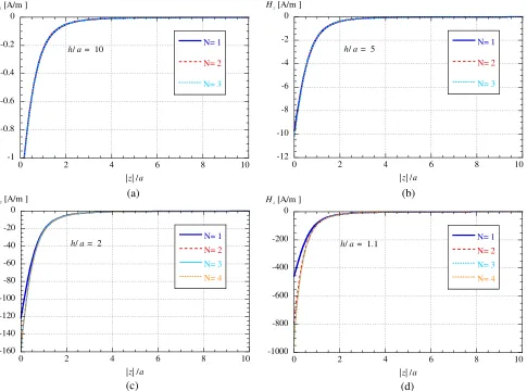
Figure 4. Scattered magnetostatic field along the z axis (ρ = 0) as a function of |z|/a for different values of h/a. (a) h/a = 10; (b) h/a = 5; (c) h/a = 2; (d) h/a = 1.1. The curves are superimposed from N = 1 in (a) and (b), from N = 2 in (c), and N = 3 in (d). Parameters: a= 5 cm,|m|= 1 Am2.
The excellent convergence properties of the basis functions and the behavior of the magnetostatic field along thez axis as a function of the ratio|z|/a for different values of h/aare reported in Fig. 4.
It is worth noting that for sources sufficiently far from the disk,only one basis functionis sufficient to reach an excellent convergence so that in these cases
Hzscat(0, z)i1
√ a (|z|2+a2)3/4P
−3/2 1/2
|z|
|z|+a2
(85)
where
i1=−| m|
π 2Γ
2 +1
2
Γ
2− 1 2
√ 1
a(a2+h2)3/4P −3/2 1/2
h
|h|2+a2
(86)
By letting
cosθz = |z|
|z|2+a2, cosθh= h
and using Eq. (55) we thus obtain
Hzscat(0, z) −3|m| π
P1−/32/2(cosθh)
(a2+h2)3/4
P1−/32/2(cosθz)
(|z|2+a2)3/4 (88)
so that the total magnetostatic field along the symmetry axis is
Hztot(0, z) |m| 2π
⎧ ⎨ ⎩
1
(|z−h|)3 −6
P1−/32/2(cosθh)
(a2+h2)3/4
P1−/32/2(cosθz)
(|z|2+a2)3/4 ⎫ ⎬
⎭ (89)
The magnetostatic shielding effectiveness SEH along the z axis can thus be evaluated as
SEH = 20 logH inc z (0, z) |Htot
z (0, z)|
(90)
Some numerical results for a disk with a= 5 cm are reported in Fig. 5.
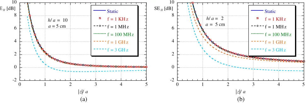
It is very interesting to note that the static approximation provides accurate results up to relatively high frequencies. In Fig. 6 the static and exact frequency-dependent magnetic shielding effectiveness SEH are reported for different frequencies and observation points for the cases h/a= 10 and h/a= 2.
0 5 10 15 20
0 1 2 3 4
h/a = 10
h/a = 5
h/a = 2
h/a = 1.1
|z| /a SE [dB]
5
Figure 5. Magnetostatic shielding effectiveness SEH along the semi-axis z <0 as a function of |z|/a for different values ofh/a. Parameters: a= 5 cm.
-2 0 2 4 6 8 10
0 1 2 3 4 5
Static
f = 1 KH z
f = 1 MH z
f = 100 MH z
f = 1 GH z f = 3 GH z
|z|/a
SE [dB]
h/a = 10
a = 5 cm
-2 0 2 4 6 8 10
0 1 2 3 4
Static f = 1 KH z
f = 1 MH z
f = 100 MH z
f = 1 GH z f = 3 GH z
|z|/a
SE [dB]
h/a = 2
a = 5 cm
5
(a) (b)
The exact frequency-dependent magnetic shielding effectiveness has been obtained through Eqs. (45) and (50) with ρ= 0.
5. APPLICATION OF THE METHOD OF ANALYTICAL REGULARIZATION (MAR)
It is interesting to observe that the proposed solution can be effectively put in the framework of the method of analytical regularization (MAR) [9, 15]. In fact, the set of dual integral equations which solve the problem is
∞
0 ˜
JSφ(λ)J1(λρ)λdλ= 0, ρ > a
∞
0 ˜
JSΦ(λ)J1(λρ) kz λdλ=
|m| 2π
∞
0 λ kze
−jkzhJ
1(λρ)λdλ , ρ < a
(91)
with basis functions given by Eq. (23) whose Hankel transform are expressed in Eq. (24). The latter are orthogonal in the rangeλ∈(0,+∞), i.e.,
∞
0
˜bm(λ) ˜bn(λ) dλ=δmn (92)
Therefore, as already discussed, by letting
JSφ(λ) = +∞
n=1
inbn(λ) (93)
the first equation in (91) is automatically satisfied. In the static limit, the weight function in the left-hand side of the second of (91) becomes
1 kz −→
j
λ (94)
and the second equation in Eq. (91) can be divided in a static and a dynamic part by expressing 1
kz = j
λ+ Ω (λ) (95)
where
Ω (λ) =
1
k2 0−λ2
− j λ
(96)
Thanks to such an extraction and to the expansion in Eq. (93), the static part of the second equation in Eq. (91) can be diagonalized and analytically inverted by using the transform in Eq. (24) and the orthogonality property of the Bessel functions in Eq. (92). In particular, following the procedure used in the application of the Method of Moments, we have
a
0
ρbm(ρ)
∞
0 j λ
N
n=1
in˜bn(λ)J1(λρ)λdλdρ+
a
0
ρbm(ρ)
∞
0
Ω (λ) N
n=1
in˜bn(λ)J1(λρ)λdλdρ=
−
a
0 ρbm (ρ)
∞
0
|m|λ 2πkze
−jkzhJ
1(λρ)λdλdρ, m= 1, . . . , N
(97)
i.e.,
j N
n=1 in
∞
0 ˜
bm(λ) ˜bn(λ) dλ+ N
n=1 in
∞
0
˜bm(λ) Ω (λ) ˜bn(λ)λdλ=−
∞
0 ˜
bm(λ)|m|λ 2
2πkz e −jkzhd
λ (98)
form= 1, . . . , N and therefore
jim+ N
n=1 in
∞
0
˜bm(λ) ˜bn(λ) Ω (λ)λdλ=−
∞
0 ˜
bm(λ)|m|λ 2
2πkz e
which can also be expressed as
im+ N
n=1
inZˆmn = ˆVm (100)
where
ˆ
Zmn=−j
∞
0
˜bm(λ) ˜bn(λ) Ω (λ)λdλ (101)
and
ˆ Vm = j
∞
0
˜bm(λ)|m|λ2 2πkz e
−jkzhdλ (102)
We thus have a matrix equation of the kind
[im] +
ˆ Zmn
[in] = [Vm] (103)
Since the asymptotic expansion of the Bessel functions for large orders results in [20] [20]
Jν(z)∼ √1 2πν
ez
2ν ν
(104)
it is immediate to recognize that
∞
m,n=1
Zˆmn2 <+∞ (105)
i.e., the operator
ˆ Zmn
is compact in the space 2 of the square-summable sequences. Since it is also [Vm]∈2, it follows that (100) is a second-kind Fredholm equation in 2 of the kind
X+AX=B (106)
Thanks to the Fredholm theory [23], this means that the exact solution
X= (I+A)−1B (107)
certainly exists, where I is the identity operator, and that the solution of the discretized problem converges to such an exact solution in the point-wise sense. In practice, the solution of the system truncated to a finite number N of equations converges to the exact solution. This means that if X(N) is the solution of the truncated system
X(N)+A(N)X(N)=B(N) (108) then the relative error, by the norm in2, is limited as
e(N) = ||X−X (N)||
||X|| ≤ ||(I+A) −1||||
A−A(N)|| (109)
and vanishes asN → ∞.
6. CONCLUSION
The electromagnetic field of a vertical magnetic dipole shielded by an infinitesimally thin perfectly conducting disk has been evaluated in an exact form.
regularization. Finally, the static-limit solution has been extracted in a closed form which has been shown to be accurate up to sufficiently high frequencies.
Possible generalizations of the proposed approach could address the treatment of thin disks with a finite conductivity or/and sources displaced from the symmetry axis of the disk. In both cases the problem would remain planar (whereas a non-negligible thickness of the disk would radically change the mathematical nature of the problem); in the former case, a surface transition impedance boundary condition should be enforced; in the latter case, a representation of the displaced source in terms of continuous, azimuthally phased ring sources should be employed, and the scattered field would be hybrid (TMz/TEz). Consideration of such generalized problems will be the subject of future work.
REFERENCES
1. Bethe, H. A., “Theory of diffraction by small holes,” Phys. Rev., Vol. 66, No. 7–8, 163, 1944. 2. Bouwkamp, C., “On the diffraction of electromagnetic waves by small circular disks and holes,”
Philips Research Reports, Vol. 5, 401–422, 1950.
3. Eggimann, W., “Higher-order evaluation of dipole moments of a small circular disk,” IRE Trans. Microw. Theory Techn., Vol. 8, No. 5, 573–573, 1960.
4. “Higher-order evaluation of electromagnetic diffraction by circular disks,” IRE Trans. Microw. Theory Techn., Vol. 9, No. 5, 408–418, 1961.
5. Williams, W., “Electromagnetic diffraction by a circular disk,”Proc. Cambridge Phil. Soc., Vol. 58, No. 4, 625–630, Cambridge University Press, 1962.
6. Jones, D., “Diffraction at high frequencies by a circular disc,”Proc. Cambridge Phil. Soc., Vol. 61, No. 1, 223–245, Cambridge University Press, 1965.
7. Marsland, D., C. Balanis, and S. Brumley, “Higher order diffractions from a circular disk,” IEEE Trans. Antennas Propag., Vol. 35, No. 12, 1436–1444, 1987.
8. Duan, D.-W., Y. Rahmat-Samii, and J. Mahon, “Scattering from a circular disk: A comparative study of PTD and GTD techniques,” Proc. IEEE, Vol. 79, No. 10, 1472–1480, 1991.
9. Nosich, A. I., “The method of analytical regularization in wave-scattering and eigenvalue problems: Foundations and review of solutions,” IEEE Antennas Propag. Mag., Vol. 41, No. 3, 34–49, 1999. 10. Bliznyuk, N. Y., A. I. Nosich, and A. N. Khizhnyak, “Accurate computation of a circular-disk
printed antenna axisymmetrically excited by an electric dipole,”Microw. Opt. Techn. Lett., Vol. 25, No. 3, 211–216, 2000.
11. Hongo, K. and Q. A. Naqvi, “Diffraction of electromagnetic wave by disk and circular hole in a perfectly conducting plane,” Progress In Electromagnetics Research, Vol. 68, 113–150, 2007. 12. Balaban, M. V., R. Sauleau, T. M. Benson, and A. I. Nosich, “Dual integral equations technique
in electromagnetic wave scattering by a thin disk,”Progress In Electromagnetics Research, Vol. 16, 107–126, 2009.
13. Hongo, K., A. D. U. Jafri, and Q. A. Naqvi, “Scattering of electromagnetic spherical wave by a perfectly conducting disk,”Progress In Electromagnetics Research, Vol. 129, 315–343, 2012. 14. Di Murro, F., M. Lucido, G. Panariello, and F. Schettino, “Guaranteed-convergence method of
analysis of the scattering by an arbitrarily oriented zero-thickness PEC disk buried in a lossy half-space,” IEEE Trans. Antennas Propag., Vol. 63, No. 8, 3610–3620, 2015.
15. Nosich, A. I., “Method of analytical regularization in computational photonics,”Radio Sci., Vol. 51, No. 8, 1421–1430, 2016.
16. Lucido, M., G. Panariello, and F. Schettino, “Scattering by a zero-thickness PEC disk: A new analytically regularizing procedure based on Helmholtz decomposition and Galerkin method,” Radio Sci., Vol. 52, No. 1, 2–14, 2017.
17. Chew, W. C.,Waves and Fields in Inhomogenous Media, IEEE Press, Piscataway, NJ, 1999. 18. Tango, W. J., “The circle polynomials of Zernike and their application in optics,” Appl. Phys.,
19. Rdzanek, W., “Sound scattering and transmission through a circular cylindrical aperture revisited using the radial polynomials,”J. Acoust. Soc. Am., Vol. 143, No. 3, 1259–1282, 2018.
20. Gradshteyn, I. S. and I. M. Ryzhik,Table of Integrals, Series, and Products, 7th Edition, Academic Press, Burlington, MA, 2014.
21. Jackson, J. D.,Classical Electrodynamics, 3rd Edition, Wiley, New York, 199.
22. Eason, G., B. Noble, and I. N. Sneddon, “On certain integrals of Lipschitz-Hankel type involving products of Bessel functions,” Phil. Trans. R. Soc. Lond. A, Vol. 247, No. 935, 529–551, 1955. 23. Reed, M. and B. Simon, Method of Modern Mathematical Physics, Vol. 1: Functional Analysis,