A numerical tool for predicting the spatial decay of freestream turbulence.

(1)

Scholarship@Western

Electronic Thesis and Dissertation Repository

4-12-2018 10:00 AM

A numerical tool for predicting the spatial decay of freestream

turbulence.

Dwaipayan Sarkar

The University of Western Ontario

Supervisor Savory, Eric

The University of Western Ontario

Graduate Program in Mechanical and Materials Engineering

A thesis submitted in partial fulfillment of the requirements for the degree in Master of Engineering Science

Follow this and additional works at: https://ir.lib.uwo.ca/etd

Part of the Other Mechanical Engineering Commons

Recommended Citation Recommended Citation

Sarkar, Dwaipayan, "A numerical tool for predicting the spatial decay of freestream turbulence." (2018). Electronic Thesis and Dissertation Repository. 5331.

https://ir.lib.uwo.ca/etd/5331

This Dissertation/Thesis is brought to you for free and open access by Scholarship@Western. It has been accepted for inclusion in Electronic Thesis and Dissertation Repository by an authorized administrator of

(2)

i

The present numerical work is an attempt towards modelling of freely decaying

homogeneous isotropic turbulence with its application in experimental modelling of the

effect of incident turbulence on flow around 2D and 3D bluff-bodies. Both steady, Reynolds

Averaged Navier Stokes (RANS) and unsteady, Large Eddy simulation (LES), 3-D

numerical computational fluid dynamics (CFD) techniques have been employed to

characterise the inviscid decay of large-scale turbulence in terms of the characteristic rms

turbulent velocity fluctuations (u′) and the local integral length scale (Lu). The large-scale turbulent properties extracted from the current numerical simulations are inter-related and are

shown to behave predominantly as Saffman turbulence, which states u̅̅̅̅′2Lu3 ≈ constant. The other focus from the current study was on modelling inlet conditions for bluff-bodies in a

freestream flow. A set of three-correlation equations are formulated based on the large-scale

turbulent properties that are effective in estimating the initial and local freestream turbulence

conditions. The set of prediction equations can be deemed useful for researchers developing

wind-tunnel models in the presence of freestream turbulence. Additionally, the set of

equations is also reliable in determining appropriate near-constant turbulent conditions based

on the upstream inlet conditions. The current study aims at designing the region of constant

turbulent properties of a desired magnitude that can be helpful for boundary layer and heat

transfer studies over a bluff-body.

Keywords

Homogeneous, Isotropic, Reynolds Averaged Navier-Stokes (RANS), Large Eddy

Simulation (LES), Decay, Computational Fluid Dynamics (CFD), Freestream

(3)

ii

Co-Authorship Statement

This thesis has been prepared in accordance with the regulations for an Integrated-Article

format thesis, as stipulated by the School of Graduate and Postdoctoral studies at The

University of Western Ontario. This thesis includes co-authored articles and the following

passages explicitly state the contributors, and the nature and extent of their contribution.

Chapter 2: Numerical modelling of spatially decaying isotropic homogeneous

turbulence

The simulations conducted for this study were designed and carried out by D. Sarkar, with

the assistance of E. Savory. The text was primarily written by D. Sarkar with guidance from

E. Savory. All comparisons with literature were done by D. Sarkar, while the derivation of

the decay correlation was provided by E. Savory.

Chapter 2 will be submitted for publication under the co-authorship of Sarkar, D and Savory,

E.

Chapter 3: Comparison of RANS modelling against LES and experimental

measurements of spatially decaying isotropic homogeneous turbulence

The simulations performed for this study were carried out by D. Sarkar, with

recommendations from E. Savory. All the data processing was performed by D. Sarkar, with

guidance from E. Savory. The first draft of the text was written by D. Sarkar, whilst E.

Savory contributed to the final version of the manuscript by providing important comments

and providing recommendations for editing the text.

Chapter 3 will be submitted for publication under the co-authorship of Sarkar, D and Savory,

(4)

iii

Acknowledgments

First and foremost, I would like to express my sincere gratitude to my research supervisor Dr.

Eric Savory, who has been very supportive throughout the completion of the thesis with his

patience, valuable knowledge, feedback and constant encouragement throughout the course

of my MESc. program. This has helped me a lot to develop my learning and understanding

skills. I am thankful to him for providing me opportunities whilst allowing the room to work

in my own way. Professor Savory has always been available for constructive discussions on

my research and different other topics. Almost every time, I met him, I learned something

new. His advice on different avenues of research, as well as on my approach to graduate

studies in general, has been of great value over the past two years and I truly am grateful to

all the supports provided by him. I would also like to thank my thesis advisory committee

Professor Anthony Straatman and Professor Kamran Siddiqui. They have helped the

progression of the thesis by providing new research insights and different perspective of the

research outcomes.

I would also like to acknowledge the support, I received from my colleagues in the Advanced

Fluid Mechanics Group. They have been very supportive throughout my research progression

and always been available for discussion. I am also grateful to Dr. Shady Ali who helped me

a lot to get familiar with the different commercial CFD codes and was supportive while

working on the CFD simulations.

I would like to thank the Shared Hierarchical Academic Research Computing Network

(www.sharcnet.ca) and Compute/Calcul Canada for their facilities.

I would also like to acknowledge the financial support I received from the department of

Mechanical and Materials Engineering at Western University and Natural Sciences

Engineering Research council discovery (NSERC) discovery grants.

Last but not the least; I owe my thanks to my parents Dulal Chandra Sarkar and Luna Sarkar.

Without their mental support and constant encouragement, it would not have been possible

(5)

iv

List of Tables

Table 2.1 Spanwise and normal variation of the root-mean square of the velocity fields at the

inlet with initial condition of U̅ = 4m/s, TI =10% and Lu =0.1m ... 49

Table 2.2 Percentage variation of root-mean square velocities at the inlet plane... 50

Table 2.3 Comparison between probability density function and normal distribution... 52

Table 2.4 Properties of the different grids used in the current study ... 56

Table 2.5 Grid independence study on three different grids for steady RANS predicting the turbulent kinetic energy decay along the streamwise distance ... 58

Table 2.6 Grid independence study on three different grids for steady RANS predicting the growth of integral length scales along the streamwise centreline ... 58

Table 2.7 Grid independence study on three different grids for LES simulations predicting the turbulence kinetic energy decay at 11 points along the streamwise centreline ... 61

Table 2.8 Grid independence study on three different grids for LES predicting the growth of integral length scales at 11 points along the streamwise centreline ... 61

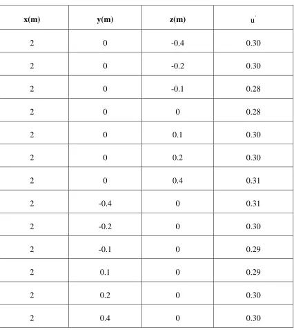
Table 2.9 Spanwise and normal variation of the root-mean square of the streamwise velocity fields at the centre plane (U̅ = 4m/s, TI = 10% and Lu = 0.10m) ... 65

Table 2.10 Overview of performed simulations on the time-step independence ... 70

Table 2.11 Summary of the virtual origin location (x0) with respect to the physical grid location for both experimental results of Kang et al. (2003) and LES ... 76

Table 2.12 Initial TKE and length scale magnitudes for experimental data of Kang et al. (2003) and the present LES study ... 77

(10)

ix

Table 2.14 Constants obtained from best regression curve fitting procedure to equations 2.49

and 2.50 using the method of Non-linear least squares ... 99

Table 2.15 Constants obtained from best regression curve fitting procedure to equation 2.60

using the method of Non-linear least squares ... 99

Table 2.16 Constants obtained from best regression fit curve procedure using the method of

Non-linear Least Squares (shift in virtual origin) ... 104

Table 2.17 Constants obtained from best regression fit curve procedure using the method of

Non-linear Least Squares (shift in virtual origin) ... 104

Table 3.1 Non-dimensional distances of the four different locations along the centreline of

the plate ... 159

Table 3.2 Comparison between the dimensionless momentum thickness, displacement

thickness and the shape factor obtained from the improved SST-k-ω model and the

theoretical laminar velocity profiles ... 168

Table 3.3 Comparisons between the dimensionless velocity shape factor obtained from the

(11)

x

List of Figures

Figure 1.1 A schematic of a typical air-based open loop BIPV/T system (adapted from

Athienitis, 2008). ... 1

Figure 1.2 Pictorial representation of a turbomachine and downstream airfoil components

(“Rolls Royce Infographic” 2014) ... 2

Figure 1.3 A schematic of the oncoming wind flow over a flat plate ... 3

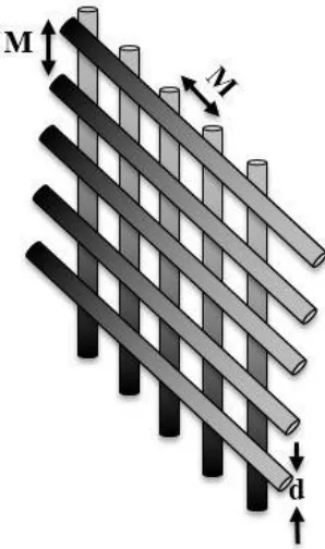
Figure 1.4 Turbulence generating grid having circular rods of diameter d and mesh width M

(adapted from Pope (2000)) ... 7

Figure 1.5 Schematic representation of the turbulence generating grid with wake vortices

being convected along the streamwise direction. The virtual origin (x0) is shown to be point where turbulence roughly re-organizes itself and complete mixing between the turbulent

structures has taken place ... 8

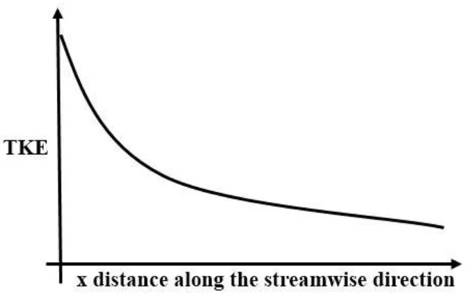
Figure 1.6 A schematic of the decay of turbulent kinetic energy in the streamwise distance x 9

Figure 2.1 Schematic of the 3D computational domain with specific boundary conditions .. 29

Figure 2.2 A schematic of the hexahedral grid distribution over the entire computational

domain... 30

Figure 2.3 Comparisons between different RANS turbulence models showing the decay of

TKE in the streamwise direction (FLUENT simulations). ... 35

Figure 2.4 Comparison between the 1st order and 2nd order discretization schemes of the SST k-ω model with respect to the spatial decay of TKE (U̅ = 4m/s, TI = 10% and Lu = 0.10m) 43

Figure 2.5 Skewness coefficient of the streamwise velocity component obtained from LES

(12)

xi

Figure 2.6 Transverse distribution of turbulence intensity laterally across the inlet plane

obtained from LES simulations with an initial condition of U̅ = 4m/s, TI = 10% and Lu = 0.10m ... 50

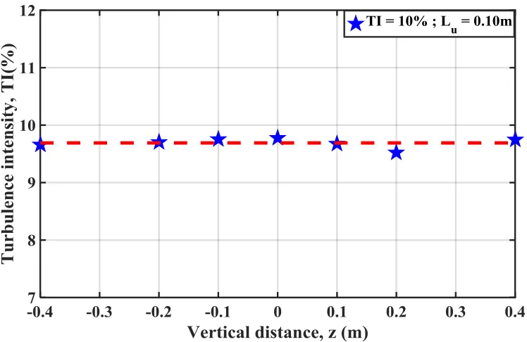
Figure 2.7 Normal Distribution of turbulence intensity vertically across the inlet plane

obtained from LES simulations with an initial condition of U̅ = 4m/s, TI = 10% and Lu = 0.10m ... 51

Figure 2.8 Kurtosis function of the streamwise velocity component obtained from LES

simulations with an initial condition of U̅ = 4m/s, TI = 10% and Lu = 0.10m ... 53

Figure 2.9 Probability density function plotted against the normal Gaussian distribution

normalized by mean velocity (U̅ = 4m/s, TI = 10% and Lu = 0.10m) ... 53

Figure 2.10 Turbulent kinetic energy spectra at the inlet plane plotted with a reference line of

slope (-5/3) representing Kolmogorov decay (U̅ = 4m/s, TI = 10% and Lu = 0.10m) ... 55

Figure 2.11 Comparison of streamwise decay of non-dimensional TKE for coarse, medium

and finer mesh (Steady RANS) (U̅ = 4m/s, TI = 10% and Lu = 0.10m) ... 57

Figure 2.12 Comparison of streamwise evolution of length scales for coarse, medium and

finer grids (Steady RANS) (U̅ = 4m/s, TI =10% and Lu = 0.10m) ... 57

Figure 2.13 Comparison of streamwise decay of non-dimensional TKE for coarse, medium

and fine grids (LES) (U̅ = 4m/s, TI = 10% and Lu = 0.10m) ... 59

Figure 2.14 Comparison of streamwise evolution of length scales for coarse, medium and

finer grids (LES) (U̅ = 4m/s, TI =10% and Lu = 0.10m) ... 60

Figure 2.15 Streamwise distribution of U̅ along the centreline normalized by the mean

velocity at the inlet i.e. U₀(U̅ = 4m/s, TI = 10% and Lu = 0.10m) ... 62

(13)

xii

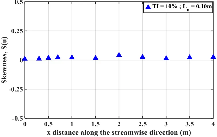
Figure 2.17 Downstream variation of velocity skewness S(u) along the centreline of the

domain (U̅ = 4m/s, TI = 10% and Lu = 0.10m) ... 66

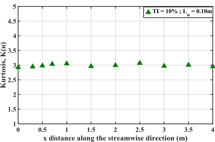
Figure 2.18 Downstream variation of Kurtosis coefficient, K(u) along the centreline of the

domain (U̅ = 4m/s, TI = 10% and Lu = 0.10m) ... 67

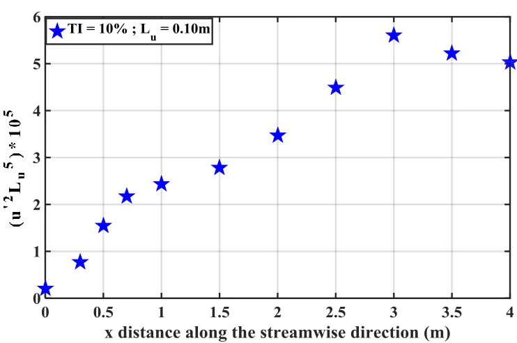
Figure 2.19 Downstream variation of '2 5 u

u L along the centreline of the domain (U̅ = 4m/s, TI

= 10% and Lu = 0.10m) ... 69

Figure 2.20 Downstream variation of u L along the centreline of the domain ('2 u3 U̅ = 4m/s, TI

= 10% and Lu = 0.10m) ... 69

Figure 2.21 Influence of the time-step size on the profiles of normalized mean velocity

component at different locations along the centreline (U̅ = 4m/s, TI = 10% and Lu = 0.10m) 71

Figure 2.22 Influence of the time step size on the streamwise turbulent kinetic energy

spectrum at the inlet (U̅ = 4m/s, TI = 10% and Lu = 0.10m) ... 72

Figure 2.23 Influence of the time-step size on the profiles of integral length scales at different

locations along the centreline (U̅ = 4m/s, TI = 10% and Lu = 0.10m) ... 73

Figure 2.24 Influence of the time-step size on the TKE decay along the centreline in the

streamwise direction (U̅ = 4m/s, TI = 10% and Lu = 0.10m) ... 74

Figure 2.25 Comparison of decay of TKE in the streamwise direction between Kang et al.

(2003) and the present LES results. ... 78

Figure 2.26 Physical distances of the virtual origin(x0) with respect to the physical grid location plotted against the ratio of physical grid element size (M/d), for all the experimental

studies of Kang et al. (2003); Krogstad & Davidson (2011); Torrano et al. (2015) ... 85

Figure 2.27 Quantitative comparisons of the spatial decay of TKE profiles between earlier

(14)

xiii

Figure 2.28 Spatial decay of TKE profiles of earlier experimental studies and present LES

study, scaled with local integral length scale (Lu) plotted with a solid line that shows the best fit power law ... 87

Figure 2.29 Spatial decay of TKE profiles for different experiments and the present LES

study scaled with initial integral length scale (Lu0) plotted with a solid line that shows the best fit power law ... 88

Figure 2.30 Comparison of the dissipation rate of turbulent kinetic energy computed as:

εq=

1 2U̅

du′2

̅̅̅̅̅̅̅

dx ) ; εiso=15ν u′2

̅̅̅̅̅

λ2 (U̅ = 4m/s, TI = 10% and Lu = 0.10m) ... 92

Figure 2.31 Ratio of the dissipation rate of turbulent kinetic energy, ε_εiso

q (U

̅_{= 4m/s, TI = 10%}

and Lu = 0.10m) ... 93

Figure 2.32 Streamwise distribution of D along the centreline of the domain obtained from

q q _{' 3}

u

D

(u ) L



 and _iso iso

' 3 u D (u ) L 

 ... 94

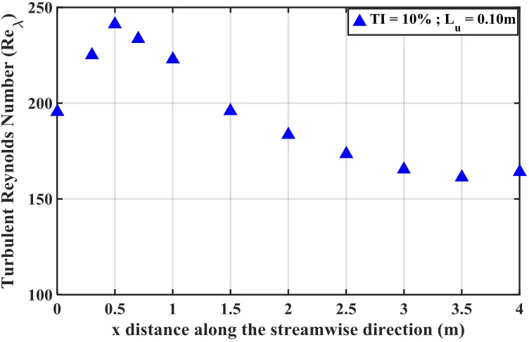
Figure 2.33 Variation of the dimensionless dissipation constant D along the streamwise

distance of the domain plotted to compare with the variation of the turbulent Reynolds

number (Rλ) along the same direction ... 96

Figure 2.34 Spatial decay of TKE profiles for different experiments and the present LES data

with the x abscissa scaled with local k and Lu plotted with a sold line that shows the best fit linear curve... 98

study scaled with local integral length scale (Lu) with a different choice of virtual origin (x0) plotted with a solid line that shows the best fit power law ... 101

(15)

xiv

study scaled with local TKE (k) and local integral length scale (Lu), with a different choice of virtual origin(x0) plotted with a solid line that shows the best fit power law ... 103

Figure 2.38 Spatial decay of TKE profile (LES) plotted against the streamwise distance x (U̅

= 4m/s, TI = 10% and Lu = 0.10m) ... 107

Figure 2.39 Rate of spatial decay of TKE profile (LES) along the streamwise distance x (U̅ =

4m/s, TI = 10% and Lu = 0.10m) ... 107

Figure 2.40 Rate of spatial decay of TKE profile in the form of

' 0.5

0 0 0 u

d(k / k ) / d((xx ) *(k ) / L plotted against (xx ) *(k )₀ ₀' 0.5/ L_u for all the

experimental data and the LES results (U̅ = 4m/s, TI = 10% and Lu = 0.10m) ... 108

Figure 2.41 Spatial decay of TKE profiles for different Reynolds number (Re) prescribed at

the inlet (RANS) ... 110

Figure 2.42 Spatial decay of TKE profiles (RANS) for different integral length scales (Lu) prescribed at the Inlet ... 111

Figure 2.43 Spatial Decay of TKE profiles (RANS) for different turbulence Intensities

prescribed at the Inlet ... 111

Figure 2.44 Spatial decay of TKE profiles (RANS) for different turbulence intensities and

integral length scales plotted with a solid line that shows the best fit power law ... 112

Figure 2.45 Spatial decay of TKE profiles for different integral length scales (Lu) prescribed at the inlet (LES) ... 113

Figure 2.46 Spatial decay of TKE profiles for different turbulence intensities at the inlet

(LES) ... 114

Figure 2.47 Downstream variation of u L'2 _u3/ U L2 _{u 0}3 along the centreline of the domain

(16)

xv

Figure 2.48 Spatial decay of TKE profiles for different Turbulence Intensities and Integral

length scales plotted with a solid line that shows the best fit power law... 115

Figure 2.49 Spatial decay of TKE profiles for different turbulence intensities and integral

length scales compared with the relevant experimental results plotted with a solid line that

shows the best fit power law ... 117

Figure 2.50 Spatial decay of TKE profiles for different inlet turbulence intensities (TI) and

integral length scales (Lu) along the streamwise distance x ... 118

Figure 2.51 Rate of spatial decay of TKE profiles for different inlet turbulence intensities

(TI) and integral length scales (Lu) along the streamwise distance x ... 119

Figure 3.1 Spatial decay of TKE profiles obtained from three different commercial codes

(FLUENT, STAR-CCM+ and CFX) compared with the LES and the previous experimental

studies ... 136

Figure 3.2 Spatial decay of TKE profiles obtained from the different optimized SST-k-ω

RANS model compared with the LES and the earlier experimental studies, (FLUENT

simulations) ... 142

RANS model compared with the LES and the earlier experimental studies, (FLUENT

simulations) ... 143

RANS model compared with the present LES study along the streamwise distance x

(FLUENT simulations) ... 144

RANS model compared with the present LES and the earlier experimental studies

(STAR-CCM+ simulations) ... 145

RANS model compared with the LES and the earlier experimental studies, (CFX

(17)

xvi

Figure 3.7 Spatial decay of TKE profiles from different optimized SST-k-ω model compared

with the LES and the earlier experimental studies (TI = 20%, Lu0 = 0.1m) ... 148

with the LES and the earlier experimental studies (TI = 30%; Lu0 = 0.1m) ... 149

Figure 3.10 Spatial decay of TKE profiles obtained from optimized SST-k-ω model

compared with the LES and the earlier experimental studies (TI = 10%; Lu0 = 0.1m) ... 150

Figure 3.11 Spatial decay of TKE profiles obtained from optimized SST-k-ω model

compared with the LES and the earlier experimental studies (TI = 10%; Lu0 = 0.05m) ... 150

Figure 3.12 Spatial decay of TKE profiles obtained from the optimized SST-k-ω model

compared with the LES and the earlier experimental studies (TI= 10%; Lu0 = 0.02m) ... 151

Figure 3.13 Schematic of the computational domain with the plate along with the relevant

boundary conditions ... 152

Figure 3.14 Local skin-friction profiles plotted for three different grids measured along the

centreline of the plate ... 158

Figure 3.15 Schematic of the flat plate showing the location of four different measurement

points along the centreline of the plate ... 159

Figure 3.16 Normalized velocity profile plotted for three different grids along the centreline

of the plate at x = 2.0m (right) and x = 2.5m (left) ... 160

Figure 3.18 Local skin-friction profiles plotted for three different grids measured along the

(18)

xvii

Figure 3.20 Comparison of the local skin-friction profiles obtained from the standard and the

improved SST-k-ω model plotted against the theoretical laminar skin-friction profiles,

measured along the centreline of the plate ... 164

Figure 3.21 Normalized velocity profile obtained from the standard and the improved

SST-k-ω model plotted against the theoretical laminar velocity profiles, measured along the

centreline of the plate at x = 2.0m (right) and x = 2.5m (left) ... 166

Figure 3.22 Normalized velocity profile obtained from the standard and the improved

SST-k-ω model plotted against the theoretical laminar velocity profiles, measured along the

Figure 3.23 Normalized velocity profile obtained from the standard and the improved k-kl-ω

model plotted against the theoretical turbulent velocity profiles, measured along the

Figure 3.24 Plot of normalized velocity profile in the logarithmic form obtained from the

standard and the improved k-kl-ω model measured at x = 2.5m ... 172

Figure 3.25 Plot of normalized velocity profile in the logarithmic form obtained from the

standard and the improved k-kl-ω model measured at x = 2.0m ... 172

Figure 3.26 Comparison of the local skin-friction profiles obtained from the standard and the

improved k-kl-ω model plotted against the theoretical turbulent skin-friction profiles,

(19)

xviii

List of Appendices

Appendix A - Solution method of the linear dependency of (k/k0) with (x-x0)*(k′0)0.5/Lu

………184

Appendix B - Sample calculations to estimate the initial turbulent scales (k′0) and Lu0) based on the local TKE (k) and the integral length scale (Lu)……….………188

Appendix C - Comparisons between three different commercial codes against the spatial decay of isotropic homogeneous turbulence………….……….195

Appendix D - Near-wall treatment of boundary layer………...………207

Appendix E - Low Reynolds Number modelling approach………...……210

(20)

xix

List of Abbreviations, Symbols, and Nomenclature

Latin Symbols

1

a , c SST-k-₁ ω model constants that are used to compute the turbulent

viscosity

A Decay coefficient

f

c Local skin-friction coefficient

p

c Specific heat capacity of the fluid (J/kg-K)

C_ Turbulence model constant (_* for SST-k-ω model)

k

C , C_ Model constants for LES

s

C Smagorinsky-Lilly constant

d Diameter of the round-grid elements/Bar-width (m)

D Dimensionless dissipation constant

D_ Cross -Diffusion term

D_ Positive portion of the cross-diffusion term

1 2

F , F Blending functions for the SST-k-ω turbulence model

b

G Generation of turbulent kinetic energy due to buoyancy

k

G Generation of turbulent kinetic energy due to the mean velocity

gradients

(21)

xx

h Convective heat-transfer coefficient

k Turbulent kinetic energy (m2_/s2₎

'

k Non-dimensional TKE

kl Laminar kinetic energy (m2/s2)

kP Turbulent kinetic energy at centre point P of wall-adjacent wall (m2/s2)

ksgs Sub-grid scale kinetic energy (m2/s2)

Ls Mixing-length for the sub-grid scales (m)

Lu Integral length scale of an eddy (m)

x y, z

L , L L Physical dimensions of the computational domain in x, y

and z direction

M Mesh-width (m)

n Decay exponent

Nu Nusselt number

P Centre point of the wall adjacent wall

p Pressure (Pa)

Pr Prandtl number

t

Pr Turbulent Prandtl number

d

Re Reynolds number based on the grid-dimension d

(22)

xxi L

Re Average Reynolds number based on the plate length in the

streamwise direction

ReLu0 Turbulent Reynolds number based on the integral length scale at the inlet (Lu0)

t

Re Local turbulent Reynolds number

X

Re Reynolds number based on the distance from the leading

edge of the plate

Re_ Turbulent Reynolds number based on the Taylor length scale

k

R Constant used in the low Reynolds number correction factor

for the SST-k-ω model

1

S Scalar measure of the deformation tensor

ij

S Mean rate-of-strain rate tensor

k

S User defined source term for turbulent kinetic energy

St Stanton number

S_ User defined source term for turbulence dissipation rate

S_ User defined source term for turbulence specific dissipation rate

t Flow time (s)

pv

T Temperature of the photovoltaic panel (K)

surr

T Temperature of the surroundings (K)

(23)

xxii

Tu Turbulence intensity in fraction

i

u Velocity vector component along the i-th base coordinates

(x direction)

j

u Velocity vector component along the j-th base coordinates

(y direction)

*

u Boundary-layer friction velocity (m/s)

u, v, w Velocity component in x, y, z direction (m/s)

' ' '

u , v , w Root-mean square velocity fluctuations in x, y and z direction

(m/s)

' ' '

u (t), v (t), w (t) Time-dependent velocity fluctuations in x, y and z direction (m/s)

' ' ' '

u u , v v Reynolds normal stress components (m2/s2)

' '

u v Reynolds shear stress component (m2/s2)

du/dy Streamwise velocity gradient (s-1₎

U Mean velocity (m/s)

v Velocity vector

x Distance along the streamwise direction (m)

0

x Virtual origin (m)

j

x Cartesian coordinate component along the j-th base vector

X Distance from the leading edge of the plate (m)

k

(24)

xxiii M

Y Contribution of the fluctuating dilatation in compressible

turbulence to the overall dissipation rate

Y_ Dissipation of ω due to turbulence

y Distance from the closest no-slip wall in the normal direction (m)

P

y Distance (normal) of centre point P of wall-adjacent cell to the wall

(m)

y Dimensional wall normal distance

Greek symbols

*

 Coefficient for Low-Reynolds number correction for

the SST-k-ω turbulence model

* i

,

 _ Constants used in computation of *

 Local grid scale (m)

t

 Time-step (s)

x. y, z

   Grid-cell size (m)

T

 Temperature difference (K)

 Turbulent kinetic energy dissipation rate (m2/s3)

 Wave-number of an eddy/Von-Kármán constant

 Dynamic viscosity (N-s/m2)

t

 Turbulent viscosity (N-s/m2)

(25)

xxiv  Density (kg/m3)

 Taylor micro-length scale (m)

ij

 Stress tensor due to molecular viscosity (N/m2)

k

 Turbulent Prandtl number of turbulent kinetic energy



 Turbulent Prandtl number of turbulent dissipation rate



 Turbulent Prandtl number of turbulent specific

dissipation rate

 Specific dissipation rate of turbulent kinetic energy (s-1)

ij

 Sub-grid scale stresses (N/m2)

kk

 Isotropic part of the sub-grid scale stresses (N/m2₎

 Boundary layer thickness (m)

 Momentum thickness (m)

* n, k1, k2, 1, 2, n, 1, 2, , 1, 2

           SST-k-ω model constants

Abbreviations

ABL Atmospheric Boundary Layer

BIPV/T Building Integrated Photo-voltaic/Thermal systems

CFD Computational Fluid Dynamics

CFL Courant–Friedrichs–Lewy condition

(26)

xxv

COST European Cooperation in Science and Technology

DNS Direct Numerical Simulation

LES Large Eddy Simulation

LRC Low Reynolds Number Correction

LRNM Low Reynolds Number Modelling

PISO Pressure-Implicit with Splitting of Operators

PV Photovoltaic

PV/T Photovoltaic/Thermal

RANS Reynolds-Averaged Navier Stokes

RSM Reynolds Stress Model

SIMPLE Semi-Implicit Method for Pressure-Linked Equations

SST Shear-Stress Transport

TKE Turbulent Kinetic Energy

WF Wall Function

(27)

Chapter 1

1

Introduction

1.1 General Introduction

The performance of thermally integrated solar panel systems e.g. (building integrated

photo-voltaic thermal system (BIPV/T)) largely depends on the way the atmospheric

wind interacts with these panels. It is mainly due to the surface roughness of the ground

and abrupt bluff-body obstructions, that the incident wind profiles on these panels are

highly intermittent, turbulent and fluctuating in nature. The exterior layer of a (BIPV/T)

represents a smooth surface according to ASHRAE classification (ASHRAE (American

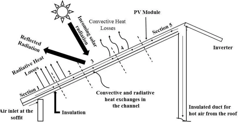
Society of Heating Refrigerating and Air-Conditioning Engineers), 2009). Figure (1.1) is a schematic of the BIPV/T system and the heat transfer terms responsible for heat transfer

over the panels.

Figure 1.1 A schematic of a typical air-based open loop BIPV/T system (adapted

from Athienitis, 2008).

Velocity and thermal boundary layers are formed at the immediate vicinity of the smooth

(28)

temperature. It is well known that boundary layers have a pronounced effect (drag, lift)

upon any object immersed in a fluid and, in many cases, they govern the dynamics of the

flow around three-dimensional bluff bodies, such as a cylinder (Geidt, (1951); Kestin &

Maeder, (1957); Smith, (1964); Bearman & Morel, (1983)) or sphere (Moradian et al.,

2009). The effect of turbulent free stream fluctuations on the boundary layer development

and its characterization is important in many thermal engineering applications such as

turbomachinery, reactors and the combustion chamber of engines. There are a number of

practical industrial situations where the boundary layers evolve differently in the

presence of an external free stream having high turbulence intensities. A most common

example is turbo-machinery flow where the wake of stators interacts with the

downstream rotors whose developing boundary layers experience that oncoming

turbulence (Fig 1.2). Similar flow patterns are also observed in heat exchanger and

combustor flows. As far as these different objects are concerned, flat plates have the

advantage of developing thicker boundary layers than those developing over rotor surface

or spheres, whose structures can be analyzed, which makes it possible to consider the

mechanisms responsible for the effect of turbulence on near wall heat transfer from these

bodies (Kondjoyan et al. (2002)).

Figure 1.2 Pictorial representation of a turbomachine and downstream airfoil components (“Rolls Royce Infographic” 2014)

Figure (1.3) shows a schematic of the fundamental problem examined in this thesis where

(29)

from it. In the figure, the term ReL represents the Reynolds number of the flow based on the plate length L given by

Re_L UL



 (1.1)

where U is the mean velocity of the flow, TI represents the turbulence intensity in

percentage given by

(

' 2 2 ' 2

1

(u v ' w )

3

TI 100

U

 

  (1.2)

where u', v', w' are the r.m.s of the turbulent velocity fluctuations in each of the x, y

and z directions), Lu represents the streamwise integral length scale of an eddy, TKE represents the turbulent kinetic energy, Tsurr is the temperature of the surroundings , Tpv is the temperature of the photovoltaic thermal panel and BIPV/T represents building

integrated photo-voltaic thermal system.

Figure 1.3 A schematic of the oncoming wind flow over a flat plate

The investigation of convective modes of heat transfer has been an important aspect in

the empirical design of different geometrical structures under various external flow

conditions (Wang & Peng (1994); Ambatipudi & Rahman (2000); Tian et al. (2004)).

Convection coefficients determined analytically (Eckertf & Carlson, (1961); Foli et al.,

(2006)) and empirically (Kestin et al., (1961); Büyüktür et al., (1964); Simonich &

(30)

approximations with negligible freestream turbulence levels and invariant properties of

the fluid with temperature and pressure. The available correlations serve as a benchmark

for problems of steady, incompressible, low-speed, uniform flows over simple systems

such as smooth plane and curved surfaces. However, the correlations formulated include

negligible disturbances of the freestream flow which cannot be extended to problems of a

surrounding turbulent atmosphere.

For many years it has been recognized that the disturbances in the mean freestream flow

can alter the heat transfer rate within the boundary layer. The freestream conditions can

cause a change in the flow regime of the boundary layer and can also shift the position of

the transition point upstream. Previous experimental studies have confirmed the

augmentation in heat transfer from certain wall geometries (both plane and curved

surfaces) in the presence of freestream turbulence in the mean flow (Fage and Falkner

(1931); Comings et al. (1948); Edwards and Furber (1956); Reynolds et al. (1958); Van

Der Hegge Zijnen, (1958); Sugawara et al. (1988)).Most of these studies have also been

the subject of review articles (e.g. Kondjoyan et al. (2002)). However, due to a large

scatter in the published results (Reynolds et al. (1958); Simonich and Bradshaw, (1978);

Sugawara et al., (1988); Maciejewski and Moffat, (1992)) on the effect of freestream

turbulence on forced convective heat transfer, a fundamental challenge is presented to

correctly predict the enhanced thermal dynamics in the laminar and turbulent region of a

developing boundary layer. Earlier studies have reported that the velocity flow field in a

boundary layer, alters significantly when there is an entrainment of the freestream

turbulence into the boundary layer (Kline et al. (1960); Charnay et al. (1976)). Studies

have also shown that the thermal field is much more sensitive to the freestream

turbulence than the dynamic field (Reynolds et al. (1958); Kondjoyan et al. (2002);

Péneau et al. (2004)). A careful inspection of the previous studies leads to the fact that

there were many discrepancies and contradictions involved in the reported findings,

mainly due to the variability in the range of Reynolds number (Re), imprecise

identification of an isotropic and homogeneous field of turbulent flows, different initial

turbulent conditions and the influence of the different experimental set-ups used in those

(31)

The first experimental quantification of the effect of the freestream turbulence on a flat

plate boundary layer was carried out by Fage and Falkner, (1931) who considered the

laminar regime. Their study concluded that the laminar boundary layer mostly remains

unperturbed by the freestream turbulence. Similar results were also reported by Edwards

and Furber, (1956) who showed that that the oncoming turbulent flow had no effect on

the rate of heat transfer for a laminar boundary layer but significantly relocated the

transition point further upstream. However, studies by Dyban etal. (1977,1985) showed

an increase in local skin-friction coefficient (cf) (where cf is the ratio between the local

shear stress and the characteristic dynamic pressure given by _f w

2

c

0.5* * U

 

 ) by 56%

at low Reynolds number flow (ReL<20000) with a freestream turbulence (TI) of 12.5%, contradicting the aforementioned previous studies. Subsequently, numerous experimental

studies (Simonich and Bradshaw, (1978); Sugawara et al., (1988); Maciejewski and

Moffat, (1992); have been carried out to understand the relationship between the heat

transfer enhancement (expressed in terms of Stanton number (St) ,where Stanton number

(St) is a dimensionless number given by the ratio of the heat transferred into the fluid to

the thermal capacity of the fluid given by

p

h St

Uc



 , where h is convective heat transfer

coefficient, c is the specific heat capacity of the fluid) and the freestream turbulent _p

fluctuations (TI) within the turbulent boundary layer regime. But there was a

considerable variation in the magnitude of the heat transfer enhancement in each of those

cases. The analysis of turbulent boundary layer skin friction (cf) and heat transfer rate (St) by Blair, (1983a;1983b) showed that these effects were, indeed, a function of freestream

turbulence intensity (TI), integral length scale (Lu) (where Lu gives the average size of an energy containing eddy) and Reθ (where Reθ is the momentum thickness Reynolds

number given by Re_ U.



 , θ is the momentum thickness of the boundary layer . New

correlations for the effect of freestream turbulence on skin friction, heat transfer and the

Reynolds analogy factor were also presented by Blair (1983a ;1983b), which will be later

used in the future work for comparisons. A review by Kondjoyan et al., (2002) concluded

(32)

a turbulence level of 5% to 10% either in a laminar or turbulent boundary layer. The

alterations of the velocity log law and the law of the wake may make it possible to

explain a few of the disparities in the existing experimental results; Fage and Falkner,

(1931); Charnay et al., (1976); Dyban et al., (1977); Blair, (1983a; 1983b) Dyban et al.,

(1985)). However, Palyvos, (2008) in his study pointed out the lack of generality of the

existing heat transfer correlations relating Nusselt number (Nu), Reynolds number (Re)

and Prandtl number (Pr) and concluded that there is an obvious lack of physical

equivalence, because of the diverse experimental conditions under which they have been

measured. Test and Lessmann, (1980) and Loveday and Taki, (1996) anticipated that the

turbulence intensity (TI) of the approach flow might be one of the primary sources of

some of the discrepancies between the experimental studies. Thus, the turbulent

properties of the freestream flow approaching and passing the flat plate need to be

quantified in order to begin to understand their influence on heat transfer rates from flat

plates.

It is however, now well known that in absence of any external turbulent energy

generating source, the freestream eddy fluctuations exhibit continuous decay of kinetic

energy due to inertial eddy interactions at high Reynolds number. At low Reynolds

number the decay occurs mostly due to the molecular viscosity of the eddies. Thus, the

freestream turbulent kinetic energy (TKE) decay becomes an important factor of

consideration before invoking any heat transfer study related to it, since its decay will

have a direct effect on the evolution of the flow around any bluff body. It is hoped that

quantifying the incidence TKE over the leading edge of a flat plate will help in precise

estimation of the effect of freestream turbulence on boundary layer heat transfer in a

comprehensive manner and thereby reconcile some of the differences observed in the

earlier studies. Therefore, in the current study, attempts have been made to quantify the

streamwise decay of the freestream turbulent fluctuations in order to identify a region of

nearly uniform oncoming turbulent properties, so that any bluff body aerodynamics study

(33)

1.1.1 Grid-generated turbulence decay

Stationary grids or perforated screens are often used to generate turbulence in typical

wind-tunnel experiments where the Reynolds number (Re_d Ud



 ) based on the grid

-dimension (d) is high enough (order of few hundreds) in magnitude. Grid-generated

turbulence has served as a benchmark test case for turbulent theories and simulations

over several decades and continues to do so in the present. Turbulence generated by

grids decays downstream with a typical power-law of the form _TI _{A * (}x x0₎ n M



 

(Batchelor and Townsend, (1948), Pope, (2000)) (where x is the streamwise distance, x0 is the virtual origin, M is the mesh width, exponent n gives the decay rate and A gives the

decay coefficient for a specific grid and Reynolds number (Red)). For a better understanding of the variables related to the power law form of the grid-generated

turbulence, figures (1.4) and (1.5) have been shown which gives a clear visual

representation of the grid elements and the importance of the virtual origin (x0).

Figure 1.4 Turbulence generating grid having circular rods of diameter d and mesh

(34)

Figure 1.5 Schematic representation of the turbulence generating grid with wake

vortices being convected along the streamwise direction. The virtual origin (x0) is

shown to be point where turbulence roughly re-organizes itself and complete mixing

between the turbulent structures has taken place

However, it has been observed that different sets of geometrical grids introduce a

variation in the magnitude of the exponent (n) of the kinetic energy decay that affects the

structure of turbulence at small scales (Tan-atichat et al., (1982); Lavoie et al., (2005)).

In recent years, numerous wind tunnel experiments have been focused on generating

homogeneous turbulence by different type of grids; passive (Ishida et al., (2006);

Krogstad and Davidson, (2010)), active (Kang et al., (2003); Mordant, (2008)) and

multiscale (fractal) (Mazzi and Vassilicos, (2004), Seoud and Vassilicos, (2007), Hurst

and Vassilicos, (2007), Krogstad and Davidson, (2011)). However, from this literature,

concerning both numerical simulations and experiments, a marked scatter of the exponent

(n) in the range (-1.0: -1.4) (Mohamed and Larue, 1990) is discovered which implies

there may not be a universal state for grid turbulence decay.

It is very clear from the bluff body heat transfer studies mentioned above, that none of

those studies commented on the streamwise decay of freestream turbulence prior to the

bluff-body interaction (e.g. plate) nor do they discuss this issue while reporting the

experimental setups or heat transfer results. As pointed out by Corrsin and Kistler,

(1955), Townsend, (1956) and Mobbs, (1968), that turbulence intensity (TI), integral

(35)

quantified accurately before making any correct predictions for any interacting turbulent

mechanisms including convective heat transfer (CHTC) . Karava et al., (2011) in their

study tried to overcome the previous gaps and propose correlations for exterior

convective heat transfer coefficient for flat plates and, hence, the present work is an

implicit continuation of that study quantifying the effect of freestream decay before the

leading-edge incidence occurs. A conceptual schematic is shown in (fig. 1.6) that

illustrates the basic problem of the current investigation. The figure gives a perception of

the decay of TKE in the streamwise direction for the comprehensive understanding of the

reader.

Figure 1.6 A schematic of the decay of turbulent kinetic energy in the streamwise

distance x

1.2 Objective of the Thesis

The three main objectives of this thesis are: -

(36)

• To identify a region having negligible changes in the turbulent properties (such

as TKE and the integral length scale) along the streamwise distance.

• To highlight the differences and limitations of the different numerical CFD

formulations that are used as a computational tool to carry out the objectives and,

finally, to optimise those numerical models (if required) to have the correct

behaviour of turbulence decay.

However, it should be noted that this thesis only presents the objectives of the current

study which in turn attempts to fill the gap prior to addressing a larger objective, which is

to examine the influence of the freestream turbulence on convective heat transfer from

heated flat plate. Heat transfer studies are currently in progress and the analysis of the

results will form a part of future work.

In this research, three-dimensional (3D) based steady Reynolds Averaged Navier Stokes

(RANS) and unsteady Large Eddy Simulation (LES) formulations have been employed to

numerically predict the statistical properties of turbulent flows in order to overcome a

few of the challenges presented by experimental grid-generated turbulence. The RANS

study is expected to give quicker time-averaged results in comparison to LES but without

any instantaneous information of the flow variables, which will be provided by the

corresponding LES study. The RANS study also covers a wider range of turbulent flow

Reynolds number ( u0

L

Re ) (where u0

L

Re = ULu0

 , U is the mean velocity, Lu0 is the

inlet integral length scale and  is the kinematic viscosity of the fluid) flows that cannot

be covered in LES owing to the limiting constraint of available computational resources.

This is followed by a parametric analysis of the RANS and LES simulations to develop a

simple yet powerful predictive correlations of spatial decay of TKE using dimensionless

parameters.

1.3 Scope of the Thesis

The present thesis is aimed at studying and quantifying the streamwise decay of

(37)

the plate. Downstream evolution of turbulent kinetic energy (TKE) in the presence of

different initial turbulence intensities (TI) and inlet integral length scales (Lu) are also examined. Henceforth, a quantitative prediction methodology of the turbulence decay

mechanism is formulated that helps one to estimate both the local and initial values of the

turbulent parameters (TKE and Lu) in the flow field of the domain. Additionally, the study has been extended to identify regions of near constant TKE conditions in order to

allow bluff body studies in that region.

To this end, both 3-D steady RANS simulation and unsteady LES simulations have been

performed to evaluate the turbulent kinetic energy decay rate (TKE) downstream from

the inlet. The range of velocities covered in the RANS study are 4m/s, 10m/s, 20m/s,

30m/s, and 40m/s, whereas only one flow velocity (4m/s) has been simulated in the

current LES study. The corresponding turbulent Reynolds numbers based on the inlet

integral length scale ( u0

L

Re ) are 2.55×103, 6.38×103, 1.28×104, 1.91×104 and 2.55×104

which fall under the category of moderate turbulent Reynolds number flows. The inlet

turbulence intensities covered in this study were 10%, 20%, 30% and the range of

integral length scales specified at the inlet were from 0.02m, 0.05m and 0.10m. The

turbulent parameters were varied at the inlet to quantify their influence on the decay rate

of TKE over the domain. The range of length scales studied here are of the order of the

boundary layer thickness that would impinge the leading edge of the plate and so would

be energetic enough to perturb the dynamic and the thermal boundary layer completely,

which is part of the heat transfer study. As a part of the future work, related to heat

transfer models, only the forced convection regime with a temperature difference (ΔT) of

30K, will be studied, as including all of free and mixed convective heat transfer regimes

is outside the scope of the study and proposed as future work.

1.4 Thesis layout

The numerical study presented herein is in the form of an Integrated Article format that

includes only statistically converged results for decaying isotropic homogeneous

(38)

Chapter 2 discusses the characteristic nature of the turbulence decay in an empty

numerical grid domain and a region of nearly constant incident turbulence intensity is

identified. The freestream decay of turbulent flow field is validated with the previous

experimental and numerical studies and a new form of decay law is suggested

considering the effect of inlet turbulence intensity (TI) and length scales (Lu). Attempts have also been made to model the turbulent inlet conditions that govern the decay rate of

free stream turbulent flows and, henceforth, a set of new correlation equations

characterizing the spatial decay of isotropic homogeneous turbulence has been

formulated. A region of nearly constant incident turbulent conditions has been identified

based on the above predictive correlation model so that the aerodynamic features of any

bluff body can be suitably studied under near constant TKE conditions. Finally, a

comprehensive review of its dependence on the initial TKE and length scales is presented

that extends our understanding of the dependence of turbulence decay on the initial

conditions.

Chapter 3 solely focuses on the qualitative and quantitative differences observed between

three different CFD commercial codes while employing RANS model in the current

study. The differences are highlighted in terms of the model constants used in these codes

and the limitations of the models are brought forward. Improvements are also suggested

for these commercial CFD codes that can be used to unify the results obtained for the

streamwise decay of isotropic homogeneous turbulence from LES. Finally, results have

been presented from these improved models to validate its prediction of the flat plate

boundary layer growth in presence of negligible free stream turbulence intensity.

The Conclusions from the present work and recommendations for future work are

presented in Chapter 4.

1.5 Summary

In summary, this chapter introduces the general nature of the current problem along with

the motivation that drives the necessity of the present study to be carried out on the

freestream decay of homogeneous isotropic turbulence. The present study is expected to

(39)

presence of freestream turbulent flow. As stated earlier, the current study only analyses

the freestream decay of isotropic homogeneous turbulence, but the final goal is to

develop relationships between the upstream incident turbulent parameters (TI, Lu and Re) and the dimensionless heat transfer variables (Nusselt number (Nu), Stanton number

(St)). Currently, investigations are being carried as a part of the future work out to

identify the fundamental features of turbulent flow over a smooth flat plate, in the

presence of freestream turbulence and, therefore, that work is not presented in the

subsequent chapters. The main intent of this current chapter was to introduce the broader

topic related to the field of convective heat transfer studies with the final aim of

quantifying the nature of thermal boundary layers in presence of freestream turbulence. It

is hoped that the present study will contribute to the fields of Environmental Fluid

Mechanics and Convective Heat Transfer to enhance our understanding of the responses

of the velocity fields and the heat transfer to incident turbulence in atmospheric boundary

layer flows.

The next chapter discusses the freestream decay of turbulence downstream of grids in a

more detail, including the limitations of the existing literature and with numerical

(40)

References

ASHRAE (American Society of Heating Refrigerating and Air-Conditioning Engineers)

(2009) ‘2009 Ashrae Handbook: Fundamentals, I-P Edition’, ASHRAE Journal,

30329(404), p. 926.

Ambatipudi, K.K. and Rahman, M.M., (2000).‘Analysis of conjugate heat transfer in

microchannel heat sinks’. Numerical Heat Transfer: Part A: Applications, 37(7),

pp.711-731.

Athienitis, A. K. (2008) ‘Design of advanced solar homes aimed at net-zero annual

energy consumtion in Canada’, in 3rd International Solar Energy Society Conference

-Asia Pacific Region. Sydney, Australia, pp. 1–14.

Batchelor, G. K. and Townsend, A. A. (1948a) ‘Decay of isotropic turbulence in the initial period’, Proceedings of the Royal Society of London, Series A, Mathematical and

Physical Sciences, 193(1035), pp. 539–558.

Bearman, P. W. and Morel, T. (1983) ‘Effect of free stream turbulence on the flow around bluff bodies’, Progress in Aerospace Sciences, 20(2–3), pp. 97–123.

Blair, M. F. (1983a) ‘Influence of free-stream turbulence on turbulent boundary layer

heat transfer and mean profile development, Part I—Experimental Data’, Journal of Heat

Transfer, 105, pp. 33–40.

Blair, M. F. (1983b) ‘Influence of free-stream turbulence on turbulent boundary layer

heat transfer and mean profile development, Part II—Analysis of Results’, Journal of

Heat Transfer, 105, pp. 41–47.

Büyüktür, A.R., Kestin, J. and Maeder, P.F., (1964). 'Influence of combined pressure

gradient and turbulence on the transfer of heat from a plate'. International Journal of

Heat and Mass Transfer, 7(11), pp.1175-1186.

Charnay, G., Mathieu, J. and Comte-Bellot, G. (1976) ‘Response of a turbulent boundary

(41)

1261-1272.

Comings, E. W., Clapp, J. T. and Taylor, J. F. (1948) ‘Air turbulence and transfer processes’, Industrial and Engineering Chemistry, 40(6), pp. 1076–1082.

Corrsin, S. and Kistler, A. L. (1955) ‘Free-stream boundaries of turbulent flows’,

NACA-report-1244, pp. 1–35.

Dyban, E. P., Epik, E. Y. and Surpun, T. T. (1977) ‘Characteristics of the laminar layer with increased turbulence of the outer stream’, Int. Chem. Eng., 17(3), pp. 501–504.

Dyban, E. P., Epik, E. Y., Zuzine, in: N. and (Eds.), A. K. (1985) ‘Transferts de chaleur et hydrodynamique dans les écoulements rendus turbulents’, in Monographie Traduite du

Russe par l’I.N.R.A. Naukova Dumka, Kiev.

Eckertf, E.R.G. and Carlson, W.O., (1961). 'Natural convection in an air layer enclosed

between two vertical plates with different temperatures'. International Journal of Heat

and Mass Transfer, 2(1-2), pp.106-120.

Edwards, A. and Furber, B. (1956) ‘The influence of free-stream turbulence on heat transfer by convection from an isolated region of a plane surface in parallel air flow’,

Proc. Inst. Mech., E 170, pp. 941–954.

Fage, A. and Falkner, V. (1931a) ‘Further experiments on the flow around a circular cylinder’, Reports and memoranda (Great Britain. Aeronautical Research Committee),

(1369).

Fage, A. and Falkner, V. M. (1931b) ‘On the relationship between heat transfer and surface friction for laminar flow’, British. Aeronautical Research Council Reports and

Memoranda, 1408(London: HMSO).

Foli, K., Okabe, T., Olhofer, M., Jin, Y. and Sendhoff, B., (2006). 'Optimization of micro

heat exchanger: CFD, analytical approach and multi-objective evolutionary algorithms'.

(42)

Geidt, W. H. (1951) ‘Effect of turbulence level of incident air stream on local heat transfer and skin friction on a cylinder’, Journal of the Aeronautical Sciences, 18(11), pp.

725–730.

Hurst, D. and Vassilicos, J. C. (2007) ‘Scalings and decay of fractal-generated turbulence’, Physics of Fluids, 19, pp. 1–31.

Ishida, T., Davidson, P. a. and Kaneda, Y. (2006) ‘On the decay of isotropic turbulence’,

Journal of Fluid Mechanics, 564, pp. 455-475.

Kestin, J. and Maeder, P.F., (1957). Influence of turbulence on transfer of heat from

cylinders, NACA Tech. Note 4018, pp. 1-78.

Kestin, J., Maeder, P.F. and Wang, H.E., (1961). 'Influence of turbulence on the transfer

of heat from plates with and without a pressure gradient'. International Journal of Heat

and Mass Transfer, 3(2), pp.133-154.

Kang, H. S., Chester, S. and Meneveau, C. (2003) ‘Decaying turbulence in an

active-grid-generated flow and comparisons with large-eddy simulation’, Journal of Fluid

Mechanics, 480, pp. 129–160.

Karava, P., Jubayer, C. M. and Savory, E. (2011) ‘Numerical modelling of forced

convective heat transfer from the inclined windward roof of an isolated low-rise building

with application to photovoltaic/thermal systems systems’, Applied Thermal Engineering,

31, pp. 1950–1963.

Kline, S. J., Lisin, A. V. and Waitman, B. A. (1960) ‘Preliminary experimental

investigation of the effect of free stream turbulence on turbulent boundary layer growth’,

NACA, Technical note, D-368, pp. 1–62.

Kondjoyan, A., Péneau, F. and Boisson, H. C. (2002) ‘Effect of high free stream

turbulence on heat transfer between plates and air flows: A review of existing

experimental results’, International Journal of Thermal Sciences, 41(1), pp. 1–16.

(43)

Generated by Multi-scale Grids’, Journal of Fluid Mechanics, 32042(680), pp. 417–434.

Lavoie, P., Burattini, P., Djenidi, L. and Antonia, R. A. (2005) ‘Effect of initial

conditions on decaying grid turbulence at low Rλ’, Experiments in Fluids, 39(5), pp. 865– 874.

Loveday, D. L. and Taki, A. H. (1996) ‘Convective heat transfer coefficients at a plane

surface on a full-scale building facade’, International Journal of Heat and Mass Transfer,

39(8), pp. 1729–1742.

Maciejewski, P. K. and Moffat, R. J. (1992) ‘Heat transfer with very high free-stream

turbulence: Part I - Experimental Data’, Journal of Heat Transfer, 114, pp. 827–833.

Mazzi, B. and Vassilicos, J. C. (2004) ‘Fractal-generated turbulence’, J. Fluid Mech, 502,

pp. 65–87.

Mobbs, F. R. (1968) ‘Spreading and contraction at the boundaries of free turbulent

flows’, Journal of Fluid Mechanics, 33, pp. 227–239.

Mohamed, M. S. and Larue, J. C. (1990) ‘The decay power law in grid-generated turbulence’, Journal of Fluid Mechanics, 219, pp. 195-214.

Moradian, N., Ting, D. S. K. and Cheng, S. (2009) ‘The effects of freestream turbulence

on the drag coefficient of a sphere’, Experimental Thermal and Fluid Science. Elsevier

Inc., 33(3), pp. 460–471.

Mordant, N. (2008) ‘Experimental high Reynolds number turbulence with an active grid’,

American Journal of Physics, 76(12), pp. 1092–1098.

Palyvos, J. A. (2008) ‘A survey of wind convection coefficient correlations for building envelope energy systems’ modeling’, Applied Thermal Engineering, 28(8–9), pp. 801–

808.

Péneau, F., Boisson, H.C., Kondjoyan, A. and Djilali, N., (2004). 'Structure of a flat plate