Universal One-Way Hash Functions and Average Case Complexity
via Inaccessible Entropy
Iftach Haitner∗ Thomas Holenstein† Omer Reingold‡ Salil Vadhan§ Hoeteck Wee¶
December 11, 2014
Abstract
This paper revisits the construction of Universal One-Way Hash Functions (UOWHFs) from any one-way function due toRompel(STOC 1990). We give a simpler construction of UOWHFs, which also obtains better efficiency and security. The construction exploits a strong connection to the recently introduced notion of inaccessible entropy (Haitner et al., STOC 2009). With this perspective, we observe that a small tweak of any one-way function f is already a weak form of a UOWHF: Consider F(x, i) that outputs the i-bit long prefix of f(x). If F were a UOWHF then given a random x and i it would be hard to come up with x′ ̸= x such that F(x, i) =F(x′, i). While this may not be the case, we show (rather easily) that it is hard to sample x′ with almost full entropy among all the possible such values of x′. The rest of our construction simply amplifies and exploits this basic property.
With this and other recent works, we have that the constructions of three fundamental cryptographic primitives (Pseudorandom Generators, Statistically Hiding Commitments and UOWHFs) out of one-way functions are to a large extent unified. In particular, all three con-structions rely on and manipulate computational notions of entropy in similar ways. Pseudo-random Generators rely on the well-established notion of pseudoentropy, whereas Statistically Hiding Commitments and UOWHFs rely on the newer notion of inaccessible entropy.
In an additional result, we use the notion of inaccessible entropy for reproving the sem-inal result of Impagliazzo and Levin (FOCS 1989): a reduction from “uniform distribution” average case complexity problems to ones with arbitrary (though polynomial samplable one) distributions.
Keywords: computational complexity, cryptography, hashing, target collision-resistance, one-way functions
∗School of Computer Science, Tel Aviv University. E-mail:[email protected]. Supported by US-Israel BSF grant 2010196. Part of this research was conducted while at Microsoft Research, New England Campus.
†ETH Zurich, Department of Computer Science. E-mail: [email protected].
‡Weizmann Institute of Science. E-mail:[email protected]. Supported by US-Israel BSF grant 2006060. §School of Engineering and Applied Sciences and Center for Research on Computation and Society, Harvard University. E-mail: [email protected]. Supported by NSF grant CNS-0831289 and US-Israel BSF grants 2006060, 2010196.
Contents
1 Introduction 1
1.1 Inaccessible Entropy . . . 2
1.2 Our Constructions . . . 2
1.3 Perspective . . . 4
2 Preliminaries 5 2.1 Notation . . . 5
2.2 Random Variables . . . 5
2.3 Entropy Measures . . . 5
2.4 Hashing . . . 7
3 Inaccessible Entropy for Inversion Problems 7 4 Inaccessible Entropy from One-way Functions 11 4.1 A Direct Construction . . . 11
4.2 A More Efficient Construction. . . 15
4.2.1 Accessible Inputs ofF – Proving Claim 21 . . . 17
4.2.2 Upper Bounding the Size ofL – Proving Claim 22 . . . 18
5 UOWHFs from Inaccessible Entropy 20 5.1 The More Efficient UOWHF. . . 20
5.1.1 Gap Amplification . . . 21
5.1.2 Entropy Reduction . . . 22
5.1.3 Reducing Output Length . . . 23
5.1.4 Additional Transformations . . . 24
5.1.5 Putting Everything Together . . . 24
5.2 UOWHF via a Direct Construction . . . 26
5.2.1 Putting Everything Together . . . 29
6 Connection to Average Case Complexity 31 6.1 Preliminaries and the Impagliazzo and Levin Result . . . 31
6.1.1 Algorithms That Err . . . 31
6.1.2 Samplable Distributions . . . 32
6.1.3 Impagliazzo and Levin Result . . . 32
6.1.4 Search Problems . . . 33
6.1.5 Search Problems vs. Decision Problems . . . 33
6.1.6 The Valiant-Vazirani Lemma . . . 34
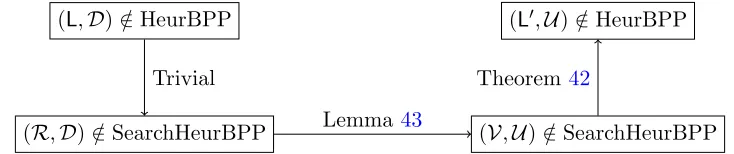
6.2 Proving Lemma 43 Via Inaccessible Entropy. . . 34
6.2.1 A Relation with Bounded Accessible Average Max-Entropy . . . 35
6.2.2 Accessible Average Max-Entropy . . . 36
6.2.3 Proving Lemma 48 . . . 37
6.2.4 A Difficult Problem For the Uniform Distribution. . . 41
1
Introduction
The following text is discussing our construction of universal one-way hash functions. Our result for average case complexity is described in Section 6.
Universal one-way hash functions (UOWHFs), as introduced by Naor and Yung [16], are a weaker form of collision-resistant hash functions. The standard notion of collision resistance requires that given a randomly chosen functionf ← F from the hash family, it is infeasible to find any pair of distinct inputs x, x′ such thatf(x) = f(x′). UOWHFs only require target collision resistance, where the adversary must specify one of the inputs x before seeing the description of the function
f. Formally:
Definition 1. A family of functions Fk =
{
Fz:{0,1}n(k)7→ {0,1}m(k)
}
z∈{0,1}k is a family of
universal one-way hash functions (UOWHFs) if it satisfies:
1. Efficiency: Givenz∈ {0,1}k andx∈ {0,1}n(k),Fz(x)can be evaluated in timepoly(n(k), k).
2. Shrinking: m(k)< n(k).
3. Target Collision Resistance: For every probabilistic polynomial-time adversary A, the proba-bility thatA succeeds in the following game is negligible ink:
(a) Let (x,state)←A(1k)∈ {0,1}n(k)× {0,1}∗. (b) Choose z← {0,1}k.
(c) Let x′←A(state, z)∈ {0,1}n(k).
(d) A succeeds if x̸=x′ and Fz(x) =Fz(x′).
It turns out that this weaker security property suffices for many applications. The most im-mediate application given in [16] is secure fingerprinting, whereby the pair (f, f(x)) can taken as a compact “fingerprint” of a large file x, such that it is infeasible for an adversary, seeing the fingerprint, to change the file x to x′ without being detected. More dramatically, Naor and Yung [16] also showed that UOWHFs can be used to construct secure digital signature schemes, whereas all previous constructions (with proofs of security in the standard model) were based on trapdoor functions (as might have been expected to be necessary due to the public-key nature of signature schemes). More recently, UOWHFs have been used in the Cramer-Shoup encryption scheme [6] and in the construction of statistically hiding commitment schemes from one-way functions [7,8].
Naor and Yung [16] gave a simple and elegant construction of UOWHFs from any one-way permutation, where Santis and Yung [21] generalized the construction of [16] to get UOWHFs fromregular one-way function. Rompel [19] gave a much more involved construction to prove that UOWHFs can be constructed from an arbitrary one-way function, thereby resolving the complexity of UOWHFs (as one-way functions are the minimal complexity assumption for complexity-based cryptography, and are easily implied by UOWHFs).1 While complications may be expected for constructions from arbitrary one-way functions (due to their lack of structure), Rompel’s analysis also feels quite ad hoc. In contrast, the construction of pseudorandom generators from one-way functions of [10], while also somewhat complex, involves natural abstractions (e.g., pseudoentropy) that allow for modularity and measure for what is being achieved at each stage of the construction.
In this paper, we give simpler constructions of UOWHFs from one-way functions, based on (a variant of) the recently introduced notion of inaccessible entropy [8]. In addition, one of the constructions obtains slightly better efficiency and security.
1.1 Inaccessible Entropy
For describing our construction, it will be cleaner to work with a variant of UOWHFs where there is a single shrinking function F :{0,1}n 7→ {0,1}m (for each setting of the security parameter k) such that it is infeasible to find collisions with random inputs. That is, an adversary A is given a uniformly random x ← {0,1}n, outputs an x′ such that F(x′) = F(x), and succeeds if x′ ̸= x.2
Note that we can assume without loss of generality that x′ = A(x) is always a preimage of F(x) (A has the option of outputting x in case it does not find a different preimage); we refer to an algorithm Awith this property as an F-collision finder.
Our construction is based on an entropy-theoretic view of UOWHFs. The fact thatF is shrink-ing implies that there are many preimagesx′ available to A. Indeed, if we consider an (inefficient) adversaryA(x) that outputsx′ ←F−1(F(x)) and letXbe a random variable uniformly distributed on {0,1}n, then
H(A(X)|X) = H(X |F(X))≥n−m,
where H(· | ·) denotes conditional Shannon entropy. (See Section 2 for more definitional details.) We refer to the quantity H(X |F(X)) as thereal entropy of F−1.
On the other hand, the target collision resistance means that effectively only one of the preimages is accessible to A. That is for every probabilistic polynomial-time F-collision finder A, we have Pr[A(X)̸=X] = neg(n), which is equivalent to requiring that:
H(A(X)|X) = neg(n)
for all probabilistic polynomial-time F-collision finders A. (If A can find a collisionX′ with non-negligible probability, then it can achieve non-non-negligible conditional entropy by outputtingX′ with probability 1/2 and outputtingX with probability 1/2.) We refer to the maximum of H(A(X)|X) over all efficient F-collision finders as the accessible entropy of F−1. We stress that accessible entropy refers to an upper bound on a form of computational entropy, in contrast to the H˚astad et al. notion ofpseudoentropy [10].
Thus, a natural weakening of the UOWHF property is to simply require a noticeable gap between the real and accessible entropies of F−1. That is, for every probabilistic polynomial-time
F-collision finderA, we have H(A(X)|X)<H(X |F(X))−∆, for some noticeable ∆, which we refer to as theinaccessible entropy of F.
1.2 Our Constructions
Our constructions of UOWHFs have two parts. First, we show how to obtain a function with no-ticeable inaccessible entropy from any one-way function. Second, we show how to build a UOWHF from any function with inaccessible entropy.
2
OWFs =⇒ Inaccessible Entropy. Given a one-way function f:{0,1}n 7→ {0,1}m, we show that a random truncation of f has inaccessible entropy. Specifically, we define F(x, i) to be the first ibits off(x).
To see that this works, suppose for contradiction that F does not have noticeable inaccessible entropy. That is, we have an efficient adversary A that on input (x, i) can sample from the set
S(x, i) ={x′:f(x′)1...i=f(x)1...i} with almost-maximal entropy, which is equivalent to sampling
according to a distribution that is statistically close to the uniform distribution onS(x, i). We can now useAto construct an inverter Invforf that works as follows on inputy: choosex0 ← {0,1}n, and then for i = 1, . . . , n generate a random xi ← A(xi−1, i−1) subject to the constraint that
f(xi)1,···,i=y1,···,i. The latter step is feasible, since we are guaranteed that f(xi)1,...,i−1=y1,···,i−1 by the fact thatAis anF-collision finder, and the expected number of trials needed get agreement with yi is at most 2 (since yi ∈ {0,1}, and y and f(xi) are statistically close). It is not difficult
to show that when run on a random output Y of f, Invproduces an almost-uniform preimage of
Y. This contradicts the one-wayness of f. Indeed, we only need f to be a distributional one-way function [13], whereby it is infeasible to generate almost-uniform preimages underf.
Inaccessible Entropy =⇒ UOWHFs. Once we have a non-negligible amount of inaccessible entropy, we can construct a UOWHF via a series of standard transformations.
1. Repetition: By evaluating F on many inputs, we can increase the amount of inaccessible entropy from 1/poly(n) to poly(n). Specifically, we take Ft(x1, . . . , xt) = (F(x1), . . . , F(xt))
where t = poly(n). This transformation also has the useful effect of converting the real entropy ofF−1 tomin-entropy.
2. Hashing Inputs: By hashing the input to F (namely taking F′(x, g) = (F(x), g(x)) for a universal hash function g), we can reduce both the real (min-)entropy and the accessible entropy so that (F′)−1 still has a significant amount of real entropy, but has (weak) target collision resistance (on random inputs).
3. Hashing Outputs: By hashing the output to F (namely taking F′(x, g) =g(F(x))), we can reduce the output length of F to obtain a shrinking function that still has (weak) target collision resistance.
There are two technicalities that occur in the above steps. First, hashing the inputs only yields weak target collision resistance; this is due to the fact that accessible Shannon entropy is an average-case measure and thus allows for the possibility that the adversary can achieve high accessible entropy most of the time. Fortunately, this weak form of target collision resistance can be amplified to full target collision resistance using another application of repetition and hashing (similar to [4]).
Second, the hashing steps require having a fairly accurate estimate of the real entropy. This can be handled similarly to [10,19], by trying all (polynomially many) possibilities and concatenating the resulting UOWHFs, at least one of which will be target collision resistant.
A More Efficient Construction. We obtain a more efficient construction of UOWHFs by hashing the output of the one-way function f before truncating. That is, we define F(x, g, i) = (g, g(f(x))1···i). This function is in the spirit of the function that Rompel [19] uses as a first step,
and enjoys a much simpler structure.3 Our analysis of this function is significantly simpler than [19]’s and can be viewed as providing a clean abstraction of what it achieves (namely, inaccessible entropy) that makes the subsequent transformation to a UOWHF much easier.
We obtain improved UOWHF parameters over our first construction for two reasons. First, we obtain a larger amount of inaccessible entropy: (logn)/nbits instead of roughly 1/n4bits. Second, we obtain a bound on a stronger form of accessible entropy, which enables us to get full target collision resistance when we hash the inputs, avoiding the second amplification step.
The resulting overall construction yields better parameters thanRompel’s original construction. A one-way function of input length n yields a UOWHF with output length ˜O(n7), improving
Rompel’s bound of ˜O(n8). Additionally, we are able to reduce the key length needed: Rompel’s original construction uses a key of length ˜O(n12), whereas our construction only needs a key of length
˜
O(n7). If we allow the construction to utilize some nonuniform information (namely an estimate of the real entropy ofF−1), then we obtain output length ˜O(n5), improvingRompel’s bound of ˜O(n6). For the key length, the improvement in this case is from ˜O(n7) to ˜O(n5). Of course, these bounds are still far from practical, but they illustrate the utility of inaccessible entropy in reasoning about UOWHFs, which may prove useful in future constructions (whether based on one-way functions or other building blocks).
1.3 Perspective
The idea of inaccessible entropy was introduced in [8] for the purpose of constructing statistically hiding commitment schemes from one-way functions and from zero-knowledge proofs. There, the nature of statistically hiding commitments necessitated more involved notions of inaccessible en-tropy than we present here — inaccessible enen-tropy was defined in [8] for interactive protocols and for “generators” that output many blocks, where one considers adversaries that try to generate next-messages or next-blocks of high entropy. In such a setting, it is necessary to have the adver-sary privately “justify” that it is behaving consistently with the honest party, and to appropriately discount the entropy in case the adversary outputs an invalid justification.
Here, we are able to work with a much simpler form of inaccessible entropy. The simplicity comes from the noninteractive nature of UOWHFs (so we only need to measure the entropy of a single string output by the adversary), and the fact that we can assume without loss of generality that the adversary behaves consistently with the honest party. Thus, the definitions here can serve as a gentler introduction to the concept of inaccessible entropy. On the other hand, the many-round notions from [8] allow for a useful “entropy equalization” transformation that avoids the need to try all possible guesses for the entropy. We do not know an analogous transformation for constructing UOWHFs. We also note that our simple construction of a function with inaccessible entropy by randomly truncating a one-way function (and its analysis) is inspired by the the construction of an “inaccessible entropy generator” from a one-way function in [8].
Finally, with our constructions, the proof that one-way functions imply UOWHFs now parallels those of pseudorandom generators [10,9] and statistically hiding commitments [7,8], with UOWHFs and statistically hiding commitments using dual notions of entropy (high real entropy, low accessible entropy) to pseudorandom generators (low real entropy, high pseudoentropy).
3[19] started with the function f′(z, g
1, g2) := (g2(f0(g1(z))), g1, g2), where g1 and g2 are n-wise independent
Paper Organization
Formal definitions are given in Section 2, where the notion of inaccessible entropy used through the paper is defined in Section 3. In Section 4 we show how to use any one-way function to get a function with inaccessible entropy, where in Section5we use any function with inaccessible entropy to construct UOWHF. Finally, our result for average case complexity is described in Section 6.
2
Preliminaries
Most of the material in this section is taken almost verbatim from [8], and missing proofs can be found in that paper.
2.1 Notation
All logarithms considered here are in base two. For t ∈ N, we let [t] = {1, . . . , t}. A function
µ:N→[0,1] is negligible, denoted µ(n) = neg(n), if µ(n) =n−ω(1). We let poly denote the set all polynomials, and let pptm denote the set of probabilistic algorithms (i.e., Turing machines) that run instrictly polynomial time.
2.2 Random Variables
LetX andY be random variables taking values in a discrete universe U. We adopt the convention that when the same random variable appears multiple times in an expression, all occurrences refer to the same instantiation. For example, Pr[X = X] is 1. For an event E, we write X|E
to denote the random variable X conditioned on E. The support of a random variable X is Supp(X) := {x: Pr[X =x]>0}. X is flat if it is uniform on its support. For an event E, we write I(E) for the corresponding indicatory random variable, i.e.,I(E) is 1 when E occurs and is 0 otherwise.
We write∥X−Y∥to denote thestatistical difference(also known as, variation distance) between
X and Y, i.e.,
∥X−Y∥= max
T⊆U|Pr[X ∈T]−Pr[Y ∈T]|
If∥X−Y∥ ≤ε(respectively,∥X−Y∥> ε), we say thatX andY areε-close [resp.,ε-far].
2.3 Entropy Measures
We will refer to several measures of entropy in this work. The relation and motivation of these measures is best understood by considering a notion that we will refer to as the sample-entropy: For a random variable X and x∈Supp(X), we define the sample-entropy of x with respect toX
to be the quantity
HX(x) := log(1/Pr[X=x]).
The sample-entropy measures the amount of “randomness” or “surprise” in the specific samplex, assuming thatxhas been generated according toX. Using this notion, we can define theShannon entropyH(X) andmin-entropy H∞(X) as follows:
H(X) := E
x←X[HX(x)]
H∞(X) := min
We will also discuss the max-entropy H0(X) := log(|Supp(X)|). The term “max-entropy” and its relation to the sample-entropy will be made apparent below.
It can be shown that H∞(X) ≤H(X) ≤ H0(X) with equality if and only if X is flat. Thus, saying H∞(X) ≥k is a strong way of saying thatX has “high entropy” and H0(X)≤k a strong way of saying thatX as “low entropy”.
Smoothed Entropies. Shannon entropy is robust in that it is insensitive to small statistical differences. Specifically, ifXandY areε-close then|H(X)−H(Y)| ≤ε·log|U|. For example, ifU =
{0,1}n and ε=ε(n) is a negligible function ofn(i.e., ε=n−ω(1)), then the difference in Shannon entropies is vanishingly small (indeed, negligible). In contrast, min-entropy and max-entropy are brittle and can change dramatically with a small statistical difference. Thus, it is common to work with “smoothed” versions of these measures, whereby we consider a random variableXto have high entropy (respectively, low entropy) ifX is ε-close to someX′ with H∞(X)≥k[resp., H0(X)≤k] for some parameterk and a negligibleε.4
These smoothed versions of min-entropy and max-entropy can be captured quite closely (and more concretely) by requiring that the sample-entropy is large or small with high probability:
Lemma 2. 1. Suppose that with probability at least 1−ε over x ← X, we have HX(x) ≥ k.
Then X is ε-close to a random variable X′ such that H∞(X′)≥k.
2. Suppose that X is ε-close to a random variableX′ such that H∞(X′)≥k. Then with proba-bility at least 1−2ε over x←X, we have HX(x)≥k−log(1/ε).
Lemma 3. 1. Suppose that with probability at least 1−ε over x ← X, we have HX(x) ≤ k.
Then X is ε-close to a random variable X′ such that H0(X′)≤k.
2. Suppose thatXisε-close to a random variableX′such thatH0(X′)≤k. Then with probability at least 1−2ε over x←X, we have HX(x)≤k+ log(1/ε).
Think of εas inverse polynomial or a slightly negligible function in n= log(|U|). The above lemmas show that up to negligible statistical difference and a slightly super-logarithmic number of entropy bits, the min-entropy [resp., max-entropy] is captured by lower [resp., upper] bound on sample-entropy.
Conditional Entropies. We will also be interested in conditional versions of entropy. For jointly distributed random variables (X, Y) and (x, y) ∈ Supp(X, Y), we define the conditional sample-entropy to be HX|Y(x |y) = log(1/Pr[X = x |Y =y]). Then the standardconditional Shannon
entropycan be written as:
H(X |Y) = E (x,y)←(X,Y)
[
HX|Y(x|y)]= E
y←Y [H(X|Y=y)] = H(X, Y)−H(Y).
There is no standard definition of conditional min-entropy and max-entropy, or even their smoothed versions. For us, it will be most convenient to generalize the sample-entropy characterizations of smoothed min-entropy and max-entropy given above. Specifically we will think of X as having “high min-entropy” [resp., “low max-entropy”] given Y if with probability at least 1−ε over (x, y)←(X, Y), we have HX|Y(x|y)≥k[resp., HX|Y(x|y)≤k].
4The term “smoothed entropy” was coined by Renner and Wolf [18], but the notion of smoothed min-entropy has
Flattening Shannon Entropy. The asymptotic equipartition property in information theory states that for independent random variablesXt= (X
1, . . . , Xt), with high probability the
sample-entropy HXt(X1, . . . , Xt) is close to its expectation. In [10] a quantitative bound on this was shown
by reducing it to the Hoeffding bound (one cannot directly apply the Hoeffding bound, because HX(X) does not have an upper bound, but one can define a related random variable which does).
We use a different bound here, which was proven in [11]. The bound has the advantage that it is somewhat easier to state, even though the proof is longer. We remark that the bound from [10] would be sufficient for our purpose (whose proof is much easier).
Lemma 4.
1. Let X be a random variable taking values in a universe U, let t∈N, and let ε >2−t. Then
with probability at least 1−ε over x←Xt,
|HXt(x)−t·H(X)| ≤O(
√
t·log(1/ε)·log(|U|))
2. Let X, Y be jointly distributed random variables where X takes values in a universe U, let
t∈N, and letε >2−t. Then with probability at least 1−εover (x, y)←(Xt, Yt) := (X, Y)t,
HXt|Yt(x|y)−t·H(X|Y)≤O(
√
t·log(1/ε)·log(|U|))
The statement follows directly from [11, Thm 2].
2.4 Hashing
A family of functionsF ={f:{0,1}n7→ {0,1}m} is2-universalif for every x̸=x′ ∈ {0,1}n, when
we choose F ← F, we have Pr[F(x) = F(x′)] ≤ 1/|{0,1}m|. F is t-wise independent if for all distinct x1, . . . , xt ∈ {0,1}n, when we choose F ← F, the random variables F(x1), . . . , F(xt) are
independent and each uniformly distributed over {0,1}m.
F isexplicitif given the description of a functionf ∈F andx∈ {0,1}n,f(x) can be computed in time poly(n, m). F is constructible if it is explicit and there is a probabilistic polynomial-time algorithm that given x∈ {0,1}n, andy ∈ {0,1}m, outputs a random f ←F such that f(x) =y.
It is well-known that there are constructible families of t-wise independent functions in which choosing a functionf ←F uses onlyt·max{n, m}random bits.
3
Inaccessible Entropy for Inversion Problems
As discussed in the introduction, for a function F, we define the real entropy of F−1 to be the amount of entropy left in the input after revealing the output.
Definition 5. Let n be a security parameter, and F:{0,1}n 7→ {0,1}m a function. We say that
F−1 has real Shannon entropy k if
H(X|F(X)) =k,
where X is uniformly distributed on {0,1}n. We say that F−1 has real min-entropy at least k if there is a negligible function ε=ε(n) such that
Prx←X
[
HX|F(X)(x|F(x))≥k ]
We say thatF−1 has real max-entropy at mostkif there is a negligible function ε=ε(n) such that
Prx←X
[
HX|F(X)(x|F(x))≤k ]
≥1−ε(n).
Note that more concrete formulas for the entropies above are:
HX|F(X)(x|F(x)) = logF−1(F(x)) H(X |F(X)) = E[logF−1(F(X))].
As our goal is to construct UOWHFs that are shrinking, achieving high real entropy is a natural intermediate step. Indeed, the amount by whichF shrinks is a lower bound on the real entropy of
F−1:
Proposition 6. If F:{0,1}n7→ {0,1}m, then the real Shannon entropy of F−1 is at least n−m, and the real min-entropy of F−1 is at least n−m−sfor any s=ω(logn).
Proof. For Shannon entropy, we have
H(X|F(X))≥H(X)−H(F(X))≥n−m.
For min-entropy, let S = {y∈ {0,1}m: Pr[f(X) =y]<2−m−s}. Then Pr[f(X) ∈ S] ≤ 2m· 2−m−s= neg(n), and for everyx such thatf(x)∈/ S, we have
HX|F(X)(x|F(x)) = log
1
Pr[X =x|F(X) =f(x)] = log
Pr[f(X) =f(x)] Pr[X =x] ≥log
2−m−s
2−n =n−m−s.
□
To motivate the definition of accessible entropy, we now present an alternative formulation of real entropy in terms of the entropy that computationally unbounded “collision-finding” adversaries can generate.
Definition 7. For a functionF:{0,1}n7→ {0,1}m, anF-collision-finderis a randomized algorithm
A such that for every x∈ {0,1}n and coin tosses r for A, we have A(x;r)∈F−1(F(x)).
Note that Ais required to always produce an inputx′ ∈ {0,1}n such that F(x) =F(x′). This
is a reasonable constraint because A has the option of outputting x′ =x if it does not find a true collision. We consider A’s goal to be maximizing the entropy of its output x′ = A(x), given a random input x. If we let Abe computationally unbounded, then the optimum turns out to equal exactly the real entropy:
Proposition 8. Let F: {0,1}n 7→ {0,1}m. Then the real Shannon entropy of F−1 equals the maximum ofH(A(X;R)|X)over all (computationally unbounded)F-collision findersA, where the random variable X is uniformly distributed in {0,1}n and R is uniformly random coin tosses for
A. That is,
H(X|F(X)) = max
Proof. The “optimal” F-collision finder A that maximizes H(A(X) | X) is the algorithm Ae that, on inputx, outputs a uniformly random element off−1(f(x)). Then
H(Ae(X;R)|X) = E[logf−1(f(X))] = H(X|F(X)).
□
The notion of accessible entropy simply restricts the above to efficient adversaries, e.g. those that run in probabilistic polynomial time (pptmfor short):
Definition 9. Let n be a security parameter and F:{0,1}n 7→ {0,1}m a function. We say that
F−1 has accessible Shannon entropy at mostk if for every pptm F-collision-finder A, we have
H(A(X;R)|X)≤k
for all sufficiently large n, where the random variable X is uniformly distributed on{0,1}n andR
is uniformly random coin tosses for A.
As usual, it is often useful to have an upper bound not only on Shannon entropy, but on the max-entropy (up to some negligible statistical distance). Recall that a random variable Z has max-entropy at mostk iff the support of Z is contained in a set of size 2k. Thus, we require that A(X;R) is contained in a set L(X) of size at most 2k, except with negligible probability:
Definition 10. Letnbe a security parameter andF:{0,1}n7→ {0,1}ma function. Forp=p(n)∈
[0,1], we say that F−1 has p-accessible max-entropyat most kif for everypptm F-collision-finder
A, there exists a family of sets {L(x)}x∈Supp(X) each of size at most 2k such that x ∈ L(x) for all
x∈Supp(X) and
Pr [A(X;R)∈ L(X)]≥1−p
for all sufficiently large n, where the random variable X is uniformly distributed on{0,1}n andR
is uniformly random coin tosses for A. In addition, if p =ε(n) for some negligible function ε(·), then we simply say thatF−1 has accessible max-entropy at mostk.
The reason that having an upper bound on accessible entropy is useful as an intermediate step towards constructing UOWHFs is that accessible max-entropy 0 is equivalent to target collision resistance (on random inputs):
Definition 11. Let F:{0,1}n 7→ {0,1}m be a function. For q = q(n) ∈ [0,1], we say that F is
q-collision-resistant on random inputs if for every pptm F-collision-finder A,
Pr[A(X;R) =X]≥q,
for all sufficiently large n, where the random variable X is uniformly distributed on{0,1}n andR
is uniformly random coin tosses for A. In addition, if q = 1−ε(n) for some negligible function
ε(·), we say thatF is collision-resistant on random inputs.
Lemma 12. Let n be a security parameter andF:{0,1}n7→ {0,1}m be a function. Then, for any
p=p(n)∈(0,1), the following statements are equivalent:
(2) F is(1−p)-collision-resistant on random inputs.
In particular, F−1 has accessible max-entropy 0 iff F is collision-resistant on random inputs.
Proof. Note that (1) implies (2) follows readily from the definition. To see that (2) implies (1),
simply take L(x) ={x}. □
While bounding p-accessible max-entropy with negligible p is our ultimate goal, one of our constructions will work by first giving a bound on accessible Shannon entropy, and then deducing a bound on p-accessible max-entropy for a value ofp <1 using the following lemma:
Lemma 13. Let n be a security parameter and F: {0,1}n 7→ {0,1}m be a function. If F−1 has accessible Shannon entropy at mostk, thenF−1hasp-accessible max-entropy at mostk/p+O(2−k/p) for anyp=p(n)∈(0,1).
Proof. Fix anypptmF-collision-finderA. From the bound on accessible Shannon entropy, we have that H(A(X;R)|X)≤k. Applying Markov’s inequality, we have
Pr
x←X,r←R
[
HA(X;R)|X(A(x;r)|x)≤k/p]≥1−p
Take L(x) to be the set:
L(x) ={x} ∪{x′: HA(X;R)|X(x′ |x)≤k/p}
We may rewriteL(x) as{x}∪{x′: Prr[A(x;r) =x′]≥2−k/p
}
. It is easy to see that|L(x)| ≤2k/p+1 and thus F−1 hasp-accessible max-entropy at most k/p+O(2−k/p). □
Once we have a bound on p-accessible max-entropy for some p <1, we need to apply several transformations to obtain a function with a good bound on neg(n)-accessible max-entropy.
Our second construction (which achieves better parameters), starts with a bound on a different average-case form of accessible entropy, which is stronger than bounding the accessible Shannon entropy. The benefit of this notion it that it can be converted more efficiently to neg(n)-accessible max-entropy, by simply taking repetitions.
To motivate the definition, recall that a bound on accessible Shannon entropy means that the sample entropy HA(X;R)|X(x′ |x) is small on average over x← X and x′ ←A(x;R). This sample
entropy may depend on both the input x and the x′ output by the adversary (which in turn may depend on its coin tosses). A stronger requirement is to say that we have upper bounds k(x) on the sample entropy that depend only onx. The following definition captures this idea, thinking of
k(x) = log|L(x)|. (We work with sets rather than sample entropy to avoid paying the log(1/ε) loss in Lemma 3.)
Definition 14. Let n be a security parameter and F:{0,1}n 7→ {0,1}m a function. We say that
F−1 has accessible average max-entropy at most k if for every pptm F-collision-finder A, there exists a family of sets {L(x)}x∈Supp(X) and a negligible function ε =ε(n) such that x ∈ L(x) for allx∈Supp(X), E[log|L(X)|]≤k and
Pr [A(X;R)∈ L(X)]≥1−ε(n),
for all sufficiently large n, where the random variable X is uniformly distributed on{0,1}n andR
We observe that bounding accessible average max-entropy is indeed stronger than bounding accessible Shannon entropy:
Proposition 15. If F−1 has accessible average max-entropy at mostk, then for every constant c,
F−1 has accessible Shannon entropy at most k+ 1/nc.
Proof. Given anF-collision-finderA, let{L(x)}be the sets guaranteed in Definition14. Let random variable X be uniformly distributed in {0,1}n, let R be uniformly random coin tosses for A, and let I be the indicator random variable forA(X;R)∈ L(X). So Pr[I = 0] = neg(n). Then:
H(A(X;R)|X)≤H(A(X;R)|X, I) + H(I)
≤Pr[I = 1]·H(A(X;R)|X, I = 1) + Pr[I = 0]·H(A(X;R)|X, I = 1) + neg(n)
≤Pr[I = 1]·E[log|L(X)| |I = 1] + Pr[I = 0]·n+ neg(n)
≤E[log|L(X)|] + neg(n)
≤k+ neg(n).
□
4
Inaccessible Entropy from One-way Functions
4.1 A Direct Construction
The goal of this section is to prove the following theorem:
Theorem 16. Let f : {0,1}n 7→ {0,1}n be a one-way function and define F over {0,1}n×[n] as F(x, i) =f(x)1,...,i−1. Then, F−1 has accessible Shannon entropy at mostH(Z |F(Z))− 641n2, where Z = (X, I) is uniformly distributed over{0,1}n×[n].
We do not know whether the functionF−1 has even less accessible Shannon entropy, (say, with a gap of Ω(1n)). However, it seems that a significantly stronger bound would require much more effort, and even improving the bound to Ω(n1) does not seem to yield an overall construction which is as efficient as the one resulting from Section 4.2. Therefore we aim to present a proof which is as simple as possible.
We begin with a high-level overview of our approach. Recall from Proposition8 the “optimal”
F-collision-finderAe that computesF−1(F(·)). The proof basically proceeds in three steps:
1. First, we show that it is easy to invertf using Ae (Lemma17).
2. Next, we show that if aF-collision-finderAhas high accessible Shannon entropy, then it must behave very similarly toAe (Lemma 18).
3. Finally, we show that if A behaves very similarly toAe, then it is also easy to invert f using
A(Lemma 19).
Step 1. Suppose we have an optimal collision finder Ae(x, i;r) that outputs a uniform random element fromF−1(F(x, i)). In order to invert an elementy, we repeat the following process: start with an arbitrary element x(0) and use Ae to find an element x(1) such that f(x(1)) has the same first bit asy. In thei’th step findx(i) such that the firstibits off(x(i)) equaly1,...,i (untili=n).
This is done more formally in the following algorithm for an arbitrary oracle CFwhich we set to Ae in the first lemma we prove. The algorithm ExtendOne does a single step. Besides the new symbolx′ which we are interested in,ExtendOnealso returns the number of calls which it did to the oracle. This is completely uninteresting to the overall algorithm, but we use it later in the analysis when we bound the number of oracle queries made by ExtendOne.
Algorithm ExtendOne
Oracle: An F-collision finder CF.
Input: x∈ {0,1}n,b∈ {0,1},i∈[n].
j:= 0
repeat
x′:=CF(x, i)
j:=j+ 1
untilf(x′)i =b return(x′, j)
InverterInv
Oracle: An F-collision finder CF.
Input: y∈ {0,1}n
x(0)←Un
fori= 1 tondo:
(x(i), j) :=ExtendOneCF(x(i−1), yi, i) done
returnx(n)
We first show that with our optimal collision finder Ae, the inverter inverts with only 2n calls in expectation (even though it can happen that it runs forever). Towards proving that, we define
p(b| y1,...,i−1) as the probability that the i’th bit off(x) equals b, conditioned on the event that
f(x)1,...,i−1 =y1,...,i−1 (or 0 iff(x)1,...,i−1=y1,...,i−1 is impossible).
Lemma 17. The expected number of calls to Ae in a random execution of InveA(y = f(x)) with
x← {0,1}n, is at most 2n.
Proof. Fix some string y1,...,i−1 in the image of F. We want to study the expected number of calls toAe(x(i−1), i) in caseF(x(i−1), i) =y1,...,i−1.
If we would knowyi, then this expected number of calls would be p(y 1
i|y1,...,i−1). Sinceyi= 0 with probabilityp(0|y1,...,i−1) we get that the expected number of calls is 1 if either of the probabilities is 0 and p(0|y1,...,i−1)·p(0|y1,...,i1 −1) +p(1|y1,...,i−1)·1|p(y1,...,i1 −1) = 2 otherwise. Using linearity of
Step 2. Given an F-collision finder A, we define ϵ(x, i) to be the statistical distance of the distribution of A(x, i;r) and the the output distribution of Ae(x, i;r) (which equals the uniform distribution overF−1(F(x, i))).
We want to show that ifA has high accessible Shannon entropy, thenA behaves very similarly toAe. The next lemma formalizes this by stating that ε(x, i) is small on average (over the uniform random choice of x∈ {0,1}n and i∈[n]). The lemma follows by applying Jensen’s inequality on the well known relationship between entropy gap and statistical distance.
Lemma 18. Assume H(A(Z))≥H(Z |F(Z))−641n2, then Ei←[n],x←{0,1}n[ε(x, i)]≤ 81n.
Proof.
(Z,Ae(Z))−(Z,A(Z))= E
z←Z[
(z,Ae(z))−(z,A(z))]
≤ E
z←Z[
√
H(Ae(z))−H(A(z))]
≤
√ E
z←Z[H(
e
A(z))−H(A(z))]
≤ 1
8n.
The first inequality uses the fact that if W is a random variable whose support is contained in a set S and U is the uniform distribution on S, then ∥U −W∥ ≤ √H(U)−H(W) (see [5, Lemma 11.6.1]). The second inequality follows by Jensen’s inequality. The final inequality uses H(Ae(Z)) =
H(Z |F(Z)) (Proposition 8). □
Step 3. We have seen now thatInvAe inverts f with 2n calls in expectation and that Abehaves similarly as Ae. We now want to show that InvA also inverts f efficiently. The main technical difficulty is that even though InvAe makes 2n calls to Ae in expectation and A and Ae are close in statistical distance, we cannot immediately deduce an upper bound on the number of calls InvA
makes to A. Indeed, our analysis below exploits the fact that Inv and ExtendOne have a fairly specific structure.
We find it convenient to assume PrR[A(x, i;R) =Ae(x, i;R)] = 1−ϵ(x, i), whereAe is an optimal
collision finder as above. This is always possible since we do not requireAe to be polynomial time, and also because we allow us to extend the number of random bitsAuses (we assume it just ignores unused ones). To do this,Ae first computes the statistics ofAon input (x, i), and also the result of
A(x, i;r). He checks whetherA(x, i;r) is one of the elements which occur too often, and outputs a different, carefully chosen one, with appropriate probability if this is the case.
We now show that in most executions of ExtendOne it does not matter whether we useA orAe
(that is, ExtendOne makes the same number of oracle queries to A and Ae, and outputs the same value).
Lemma 19. For any (x, i)∈ {0,1}n×[n], and any yi∈ {0,1}, we have
Pr
R[ExtendOne
A(x, y
i, i;R) =ExtendOneeA(x, yi, i;R)]≥1−
2ε(x, i)
p(yi |y1,...,i−1)
Note that the oracle algorithm ExtendOne is deterministic, and in the above expressions, R
refers to the coin tosses used by the oracles that ExtendOnequeries, namely A and eArespectively. We stress that the lemma says that both the value x′ and the number j returned are equal with high probability.
Proof. Let J = J(R) be the second coordinate of the output of ExtendOneA(x, yi, i;R) (i.e., the
counter) and Je=Je(R) the analogous output of ExtendOneAe(x, yi, i;R). We write
Pr
R[ExtendOne A(x, y
i, i;R) =ExtendOneeA(x, yi, i;R)] =
∑
j≥1 Pr
R[min(J,
e
J) =j]·Pr
R[ExtendOne A(x, y
i, i;R) =ExtendOneeA(x, yi, i;R)|min(J,Je) =j]
= E
j←PJ
[ Pr
R[ExtendOne A(x, y
i, i;R) =ExtendOneeA(x, yi, i;R)|min(J,Je) =j]
]
(2)
wherePJ is some distribution over the integers which, as it turns out, we don’t need to know.
Let now R′ be the randomness used by AorAe in roundj. Then,
Pr
R[ExtendOne A(x, y
i, i;R) =ExtendOneAe(x, yi, i;R)|min(J,Je) =j]
= Pr
R′
[
A(x, i;R′) =Ae(x, i;R′)|f(A(x, i;R′))i =yi∨f(Ae(x, i;R′))i =yi
]
,
because each iteration ofExtendOne uses fresh independent randomness.
Let P be the distribution over {0,1}n produced byA(x, i;R′), andP∗ be the (uniform) distri-bution produced byAe(x, i;R′). We get, forp=p(yi |y1,...,i−1) and ε=ε(x, i):
Pr
R′
[
A(x, i;R′) =Ae(x, i;R′)|f(A(x, i;R′))i =yi∨f(Ae(x, i;R′))i=yi
]
= ∑
x∈F−1(y
1,...,i)min(P(x), P ∗(x))
∑
x∈F−1(y
1,...,i)max(P(x), P
∗(x)) ≥
p−ε p+ε =
1−εp
1 +εp ≥1− 2ε
p .
Collecting the equations and inserting into (2) proves the lemma. □
Putting everything together. We can now finish the proof of Theorem 16. Consider the following random variables: let X be uniformly drawn from {0,1}n and let Y = f(X). Run
InvA(Y) andInvAe(Y) in parallel, using the same randomness in both executions. LetXe(0), . . . ,Xe(n)
be the random variables which have the values assigned tox(0), . . . , x(n) in the run ofInveA. Finally, let the indicator variables Qi be 1, iff the i’th call to ExtendOne in the above parallel run is the
We proceed to obtain an upper bound on Pr[Qi= 1]. Observe that for all x∈ {0,1}n:
Pr[Qi = 1|Xe(i−1) =x]
= Pr[ExtendOneA(x, Yi, i;R)̸=ExtendOneAe(x, Yi, i;R)|Xe(i−1)=x]
= ∑
yi∈{0,1}
p(yi |f(x)1,...,i−1)·Pr[ExtendOneA(x, yi, i;R)̸=ExtendOneeA(x, yi, i;R)]
≤ ∑
yi∈{0,1}
p(yi |f(x)1,...,i−1)·
2ϵ(x, i)
p(yi |f(x)1,...,i−1)
= 4ϵ(x, i)
where the inequality above follows by Lemma19. Averaging overx, we have that for alli= 1, . . . , n:
Pr[Qi= 1]≤4 E
x←{0,1}n[ϵ(x, i)] (3)
Here, we use the fact that by induction oni, the random variableXei, fori∈ {0, . . . , n}, is uniformly distributed in {0,1}n (it is uniform preimage of a uniformly chosen output). Using Equation (3), we have
Pr [ n
∑
i=1
Qi≥1
] =
n
∑
i=1
Pr[Qi= 1]
=n· E
i←[n],x←{0,1}n[Qi]
≤4n· E
i←[n],x←{0,1}n[ε(x, i)]
≤ 1
2
where the last inequality follows from Lemma 18. Hence, with probability 12, a run of InvA and
InveA produce the same output and use the same number of queries to the oraclesA. Moreover, the probability thatInvAe uses more than 8noracle queries is at most 14 (by applying Markov’s inequality on Lemma 17). Hence, with probability 14, InvA inverts f using 8n oracle queries in total, which contradicts the one-wayness off. In order to make sure thatInvA runs in polynomial time, we just halt it after 8ncalls.
4.2 A More Efficient Construction
The following theorem shows that a simplified variant of the first step of [19] (which is also the first step of [14]) yields inaccessible entropy with much stronger guarantees than those obtained in Section4.1. The function we construct is F(x, g, i) = (g(f(x))1,...,i, g), where g :{0,1}n7→ {0,1}n
Theorem 20(Inaccessible average max-entropy from one-way functions). Letf:{0,1}n7→ {0,1}n be a one-way function and let G = {g:{0,1}n7→ {0,1}n} be a family of constructible, three-wise
independent hash functions. Define F over Dom(F) :={0,1}n× G ×[n] by
F(x, g, i) = (g(f(x))1,...,i, g, i).
Then, for every constant d > 0, F−1 has accessible average max-entropy at most H(Z | F(Z))− (dlogn)/n, where Z is uniformly distributed overDom(F).
Proof. Letcbe a sufficiently large constant (whose value to be determined later as a function of the constantdin the theorem statement). The sets{L(x, g, i)}x∈{0,1}n,i∈[n],g∈G realizing the inaccessible
entropy ofF−1 are defined by
L(x, g, i) ={(x′, g, i) : f(x′)∈L˜(f(x), i)∧g(f(x′))1,...,i=g(f(x))1,...,i} (4)
where for y∈ {0,1}n and i∈[n], we let ˜
L(y, i) ={y} ∪{y′ ∈ {0,1}n: Hf(X)(y′)≥(i+c·logn) }
(5)
={y} ∪{y′ ∈ {0,1}n:|f−1(y′)| ≤2n−i/nc}.
Namely, ˜L(y, i) consists, in addition toyitself, of “i-light” images with respect tof.5 As a warm-up, it is helpful to write down ˜L(y, i) and L(x, g, i) for the case wheref is a one-way permutation.6
The proof of the theorem immediately follows by the following two claims.
Claim 21. For everypptm F-collision-finder Aand every constant c >0, it holds that
Pr[A(Z;R)∈ L/ (Z)]≤neg(n),
where Z is uniformly distributed over Dom(F) and R is uniformly distributed over the random coins of A.
Claim 22. For any constant c it holds that
E [log|L(Z)|]≤E[logF−1(F(Z))]−Ω (
clogn n
)
,
where Z is uniformly distributed in Dom(F).
□ 5Recall that the sample entropy is defined as H
f(X)(y) = log(1/Pr[f(X) =y]) =n−logf−1(y), so the “heavy”
images, wheref−1(y) is large, have low sample entropy.
6Iffis a permutation, then ˜L(y, i) is given by:
˜
L(y, i) =
{
{0,1}n ifi≤n−clogn {y} otherwise.
Then, for allx∈ {0,1}n, we have E[|L(x, G, i)|] = 2n−ifor alli≤n−clognand|L(x, g, i)|= 1 for allg∈ G and all i > n−clogn. This means that the entropy gap betweenF−1(F(Z)) andL(X, G, I) is roughly 1
n
∑
i>n−clognn−i=
4.2.1 Accessible Inputs of F – Proving Claim 21
Proof of Claim 21. Recall thatZ = (X, G, I) is uniformly distributed over Dom(F), and thatR is uniformly distributed over the random coins ofA. It suffices to show that
Pr[A1(X, G, I;R)∈/ f−1( ˜L(f(X), I))]≤neg(n) (6)
whereA1 denotes the first component ofA’s output (this holds since the other two output compo-nents of Aare required to equal (G, I), due to the fact thatF(X, G, I) determines (G, I)).
We construct an inverter Invsuch that for allF-collision-findersAand for cas in Equation (5) we have
Pr[InvA(Y)∈f−1(Y)]≥ 1
nc·Pr[A1(X, G, I;R)∈/ f
−1( ˜L(f(X), I))] (7)
whereY =f(X), and the proof of Claim 21 follows readily from the one-wayness of f.
InverterInvA
Oracle: An F-collision finder A.
Input: y∈ {0,1}n
x← {0,1}n
i←[n]
g′ ← Gy,x,i :={g∈ G:g(y)1...i=g(f(x))1...i} returnA1(x, g′, i;r)
Observe thatInvcan be implemented efficiently by samplingg′ as follows: pick first z, z∗ ∈ {0,1}n such thatz1...i =z1∗...i and use the constructibility of G to pickg withg(f(x)) =z and g(y) =z∗.
We analyze the success probability of InvA. Using the short hand notation Prg′[· · ·] for
Prg′←Gy,x,i[· · ·] we observe that
Pr[InvA(Y)∈f−1(Y)] = E
x←{0,1}n,i←[n]
[∑
y∈{0,1}nPr[f(X) =y]·gPr′,r[A1(x, g
′, i;r)∈f−1(y)]] (8)
≥ E
x,i
[∑
y /∈L˜(f(x),i) 2−i
nc ·gPr′,r[A1(x, g
′, i;r)∈f−1(y)]]
where the inequality holds since Pr[f(X) =y]≥2−i/ncfor anyy /∈L˜(f(x), i).
Next, observe that for any tuple (y, x, i) such thaty̸=f(x), it holds that (where we distinguish Prg′[· · ·] as above from Prg[· · ·] = Prg←G[· · ·])
Pr
g′,r
[
A1(x, g′, i;r)∈f−1(y)]= Pr
g←G,r
[
A1(x, g, i;r)∈f−1(y)|g(f(x))1···i =g(y)1···i
]
(9)
= Prg,r [
A1(x, g, i;r)∈f−1(y)∧g(f(x))1···i=g(y)1···i
]
Prg,r
[
g(f(x))1···i=g(y)1···i
]
= Prg,r [
A1(x, g, i;r)∈f−1(y) ]
Prg,r
[
g(f(x))1···i =g(y)1···i
]
= 2i·Pr
g,r
[
A1(x, g, i;r)∈f−1(y) ]
The second equality follows by Bayes’ rule and the third uses the fact thatAis aF-collision finder. The last equality follows since G is two-wise independent (recall we assumed that G is three-wise independent) and f(x)̸=y.
Combining the two preceding observations, and the fact that f(x)∈L˜(f(x), i), we have that
Pr[InvA(Y)∈f−1(Y)]≥ E
x←{0,1}n,i←[n]
[∑
y /∈L˜(f(x),i) 2−i
nc ·2 i· Pr
g←G,r
[
A1(x, g, i;r)∈f−1(y)]]
≥ 1
nc·x,iE
[∑
y /∈L˜(f(x),i)·Prg,r
[
A1(x, g, i;r)∈f−1(y)]]
= 1
nc·x,g,i,rPr
[
A1(x, g, i;r)∈/ f−1( ˜L(f(x), i))],
and the proof of the claim follows. □
4.2.2 Upper Bounding the Size of L – Proving Claim 22
Recall thatZ = (X, G, I) is uniformly distributed over Dom(F). In the following we relate the size of L(Z) to that of F−1(F(Z)).
We make use of the following property of three-wise independent hash-functions.
Claim 23. Let i, xandx∗, be such thatf(x)̸=f(x∗) andi≤Hf(X)(f(x∗))≤Hf(X)(f(x)). Then,
Pr
g←G z′←F−1(F(x,g,i))
[
z′ = (x∗, g, i)]≥ 2
−n
8 .
Note that in the above experiment it is always the case that (g′, i′) = (g, i), lettingz′ = (x′, g′, i′).
Proof. Note that with probability 2−i over g← G, it holds thatg(f(x∗))1···i =g(f(x))1···i.
Hence-forth, we condition on this event that we denote by E, and let w = g(f(x∗))1···i = g(f(x))1···i.
Observe that for a fixed gsatisfying E, it holds that
Pr
z′←F−1(F(x,g,i)) [
z′ = (x∗, g, i)|E]≥ 1
|F−1(F(x, g, i))| (10)
In order to obtain a lower bound on F−1(F(x, g, i)), we first consider x′ such that f(x′) ∈/
{f(x), f(x∗)}. By the three-wise independence of G,
Pr
g←G
[
g(f(x′)) =w|E]= 2−i (11)
This implies that the expected number of x′ such that g(f(x′)) = w and f(x′) ∈ {/ f(x), f(x∗)} is at most 2n−i. By Markov’s inequality, we have that with probability at least 1/2 over g ← G
(conditioned onE),
|F−1(F(x, g, i))| ≤2·2n−i+|f−1(f(x))|+|f−1(f(x∗))| ≤4·2n−i, (12)
where the second inequality uses the fact thati≤Hf(X)(f(x∗))≤Hf(X)(f(x)). Putting everything together, we have that the probability we obtainx∗ is at least 2−i·1/2·(4·2n−i)−1= 2−n/8. □