An Analysis of Affine Coordinates
for Pairing Computation
Kristin Lauter, Peter L. Montgomery, and Michael Naehrig
Microsoft Research, One Microsoft Way, Redmond, WA 98052, USA {klauter, petmon, mnaehrig}@microsoft.com
Abstract. In this paper we analyze the use of affine coordinates for pairing computation. We observe that in many practical settings, e. g. when implementing optimal ate pairings in high security levels, affine coordinates are faster than using the best currently known formulas for projective coordinates. This observation relies on two known techniques for speeding up field inversions which we analyze in the context of pairing computation. We give detailed performance numbers for a pairing imple-mentation based on these ideas, including timings for base field and ex-tension field arithmetic with relative ratios for inversion-to-multiplication costs, timings for pairings in both affine and projective coordinates, and average timings for multiple pairings and products of pairings.
Keywords:Pairing computation, affine coordinates, optimal ate pairing, finite field inversions, pairing cost, multiple pairings, pairing products.
1
Introduction
Cryptographic pairing computations are required for a wide variety of new cryp-tographic protocols and applications. All crypcryp-tographic pairings currently used in practice are based on pairings on elliptic curves, requiring both elliptic curve operations and function computation and evaluation to compute the pairing of two points on an elliptic curve [36]. For a given security level, it is important to optimize efficiency of the pairing computation, and much work has been done on this topic (see for example [6,7,5,30,35,44,42]).
In this paper we analyze the use of affine coordinates for pairing computation in different settings. We propose the use of two known techniques for speeding up field inversions and analyze them in the context of pairing computation. Based on these, we find that in many practical settings, for example when implementing one of the optimal pairings [44] based on the ate pairing [30] in high security levels, affine coordinates will be much faster than projective coordinates.
The first technique we investigate is computing inverses in extension fields by using towers of extension fields and successively reducing inverse computation to subfield computations via the norm map. We show that this technique drastically reduces the ratio of the costs of inversions to multiplications in extension fields. Thus when computing the ate pairing, where most computations take place in a potentially large extension field, the advantage of projective coordinates is eventually erased as the degree of the extension gets large. This happens for example when implementing pairings on curves for higher security levels such as 256 bits, or when special high-degree twists can not be used to reduce the size of the extension field.
The second technique we investigate is the use of inversion-sharing for pairing computations. Inversion-sharing is a standard trick whenever several inversions are computed at once. As the number of elements to be inverted grows, the average ratio of inversion-to-multiplication costs approaches 3. Inversion-sharing can be used in a single pairing computation if the binary expansion is read from right-to-left instead of left-to-right. This approach also has the advantage that it can be easily parallelized to take advantage of multi-core processors. Inversion-sharing for pairing computation can also be advantageous for computing multiple pairings or for computing products of pairings, as was suggested by Scott [41] and analyzed by Granger and Smart [25].
Ironically, although the two techniques we investigate can be used simul-taneously, it is often not necessary to do so, since either technique alone can reduce the inversion to multiplication ratio. Either technique alone makes affine coordinates faster than projective coordinates in some settings.
To illustrate these techniques, we give detailed performance numbers for a pairing implementation based on these ideas. This includes timings for base field and extension field arithmetic with relative ratios for inversion-to-multiplication costs and timings for pairings in both affine and projective coordinates, as well as average timings for multiple pairings and products of pairings. In our im-plementation, affine coordinates are faster than projective coordinates even for Barreto-Naehrig curves [8] with a high-degree twist at the lowest security levels. However, we expect that for other implementations, the benefits of affine coor-dinates would only be realized for higher security levels or for curves without high-degree twists.
Section 4 is dedicated to revisiting the well-known inversion-sharing trick and its application in pairing computation. Finally, Section 5 gives benchmarking results for our pairing implementation based on the Microsoft Research bignum library.
2
Pairing computation
Let p >3 be a prime and Fq be a finite field of characteristic p. Let E be an
elliptic curve defined overFq, given by E:y2=x3+ax+b, wherea, b∈Fq and
4a3+ 27b26= 0. We denote byOthe point at infinity onE. Letn= #E(F
q) =
q+ 1−t, wheret is the trace of Frobenius, which fulfills |t| ≤2√q. We fix a prime r withr|n. Let k be the embedding degree ofE with respect to r, i. e. k is the smallest positive integer withr|qk−1. This means that F∗
qk contains
the groupµrofr-th roots of unity. The embedding degree ofE is an important
parameter, since it determines the field extensions over which the groups that are involved in pairing computation are defined.
Form∈Z, let [m] be the multiplication-by-mmap. The kernel of [m] is the set ofm-torsion points onE; it is denoted by E[m] and we writeE(Fqℓ)[m] for
the set ofFqℓ-rationalm-torsion points (ℓ >0). Ifk >1, which we assume from
now on, we haveE[r]⊆E(Fqk), i.e. allr-torsion points are defined overFqk.
Most pairings that are suitable for use in practical cryptographic applications are derived from the Tate pairing, which is a mapE(Fqk)[r]×E(Fqk)/rE(Fqk)→
F∗
qk/(F∗qk)r (for details see [18,19]). In this paper, we focus on the ate pairing
[30], variants of which are often the most efficient choices for implementation.
2.1 The ate pairing
Given m ∈Zand P ∈E[r], letfm,P be a rational function on E with divisor
(fm,P) =m(P)−([m]P)−(m−1)(O). Letφqbe theq-power Frobenius
endomor-phism onE. Define two groups of prime orderrbyG1=E[r]∩ker(φq−[1]) =
E(Fq)[r] andG2=E[r]∩ker(φq−[q])⊆E(Fqk)[r]. The ate pairing is defined
as
aT :G2×G1→µr, (Q, P)7→fT,Q(P)(q
k
−1)/r, (1)
where T = t−1. The group G2 has a nice representation by an isomorphic group of points on a twist E′ of E, which is a curve that is isomorphic to E. Here, we are interested in those twists which are defined over a subfield of Fqk
such that the twisting isomorphism is defined overFqk. Such a twistE′ ofE is
given by an equationE′ : y2 = x3+ (a/α4)x+ (b/α6) for some α∈ F
qk with
isomorphism ψ :E′ → E, (x, y) 7→ (α2x, α3y). If ψ is minimally defined over Fqk and E′ is minimally defined over Fqk/d for a d| k, then we say that E′ is
a twist of degree d. If a = 0, let d0 = 4; if b = 0, let d0 = 6, and let d0 = 2 otherwise. Ford= gcd(k, d0) there exists exactly one twistE′ ofE of degreed for whichr|#E′(F
a group isomorphismG′
2→G2 and we can represent all elements inG2 by the corresponding preimages in G′
2. Likewise, all arithmetic that needs to be done in G2 can be carried out in G′2. The advantage of this is that points in G′2 are defined over a smaller field than those inG2. UsingG′
2, we may now view the ate pairing as a mapG′
2×G1→µr, (Q′, P)7→fT,ψ(Q′)(P)(q
k
−1)/r.
The computation ofaT(Q′, P) is done in two parts: first the evaluation of the
functionfT,ψ(Q′)atP, and second the so-called final exponentiation to the power
(qk−1)/r. The first part is done with Miller’s algorithm [36]. We describe it for
even embedding degree in Algorithm 1 which shows how to computefm,ψ(Q′)(P)
for some integerm >0. We denote the function given by the line through two pointsR1andR2onEbylR1,R2. IfR1=R2, then the line is given by the tangent to the curve passing throughR1. Throughout this paper, we assume that k is even so that denominator elimination techniques can be used (see [6,7]).
Algorithm 1Miller’s algorithm for evenkand ate-like pairings Input: Q′∈G′
2, P ∈G1, m= (1, ml−2, . . . , m0)2
Output: fm,ψ(Q′)(P) representing a class inF∗qk/(F∗qk)r
1: R′←Q′, f←1
2: forifromℓ−1 downto 0do
3: f←f2·lψ(R′),ψ(R′)(P), R′←[2]R′
4: if (mi= 1)then
5: f←f·lψ(R′),ψ(Q′)(P), R′←R′+Q′
6: end if 7: end for 8: returnf
Miller’s algorithm builds up the function valuefm,ψ(Q′)(P) in a
square-and-multiply-like fashion from line function values along a scalar multiplication com-puting [m]Q′ (which is the value of R′ after the Miller loop). Step 3 is called a
doubling step, it consists of squaring the intermediate valuef ∈Fqk, multiplying
it with the function value given by the tangent toEinR=ψ(R′), and doubling the pointR′. Similarly, an addition step is computed in Step 5 of Algorithm 1.
The final exponentiation in (1) maps classes inF∗
qk/(F∗qk)r to unique
repre-sentatives in µr. Given the fixed special exponent, there are many techniques
that improve its efficiency significantly over a plain exponentiation (see [42,24]). The most efficient variants of the ate pairing are so-called optimal ate pairings [44]. They are optimal in the sense that they minimize the size ofm and with that the number of iterations in Miller’s algorithm to log(r)/ϕ(k), where ϕ is the Euler totient function. For these minimal values ofm, the functionfm,ψ(Q′) alone usually does not give a bilinear map. To get a pairing, these functions need to be adjusted by multiplying with a small number of line function values; for details we refer to [44].
pairing-friendly, i.e. the embedding degreekneeds to be small, whilershould be larger than√q. A survey of methods to construct such curves can be found in [20]. For security reasons, the parameters need to have certain minimal sizes which lead to optimal values for the embedding degreekfor specific security levels (see for example the keysize recommendations in [43] and [4]).
Furthermore, it is advantageous to choose curves with twists of degree 4 or 6, so-called high-degree twists, since this results in higher efficiency due to the more compact representation of the group G2. To achieve security levels of 128 bits or higher, embedding degrees of 12 and larger are optimal. Because the degree of the twist E′ is at most 6, this means that when computing ate-like pairings at such security levels, all field arithmetic in the doubling and addition steps in Miller’s algorithm takes place over a proper extension field ofFq.
2.2 Costs for doubling and addition steps
In this section, we take a closer look at the costs of the doubling and addi-tion steps in Miller’s algorithm. We begin by describing the evaluaaddi-tion of line functions in affine coordinates, i.e. a point P on E, P 6= O, is given by two affine coordinates as P = (xP, yP). Let R1, R2, S ∈ E with R1 6= −R2 and R1, R26=O. Then the function of the line throughR1 and R2 (tangent toE if R1=R2) evaluated atS is given bylR1,R2(S) =yS−yR1−λ(xS−xR1), where λ= (3x2
R1+a)/2yR1ifR1=R2andλ= (yR2−yR1)/(xR2−xR1) otherwise. The valueλis also used to compute R3 =R1+R2 onE byxR3 =λ
2−x
R1−xR2 and yR3 = λ(xR1 −xR3)−yR1. If R1 = −R2, then we have xR1 = xR2 and lR1,R2(S) =xS−xR1.
Before analyzing the costs for doubling and addition steps, we introduce notations for field arithmetic costs. LetFqm be an extension of degreem ofFq
form≥1. We denote byMqm,Sqm, Iqm,addqm,subqm, andnegqm the costs
for multiplication, squaring, inversion, addition, subtraction, and negation in the field Fqm. When we omit the indices in all of the above, this indicates that we
are dealing with arithmetic in a fixed field and field extensions do not play a role. The cost for a multiplication by a constant ω ∈Fqm is denoted byM(ω).
We assume the same costs for addition of a constant as for a general addition. Let notations be as described in Section 2.1. Let e = k/d, then G′
2 = E′(F
qe)[r]. Let P ∈ G1, R′, Q′ ∈ G′
2 and let R = ψ(R′), Q = ψ(Q′). Fur-thermore, we assume thatFqk =Fqe(α) whereα∈Fqk is the same element as
the one defining the twistE′, and we haveαd =ω∈F
qe. This means that each
element inFqk is given by a polynomial of degreed−1 inαwith coefficients in
Fqe and the twisting isomorphismψmaps (x′, y′) to (α2x′, α3y′).
Doubling steps in affine coordinates: We need to compute
lR,R(P) =yP−α3yR′−λ(xP −α2xR′) =yP−αλ′xP+α3(λ′xR′−yR′)
andR′
3= [2]R′, wherexR′
3 =λ ′2−2x
R′ andyR′
3 =λ
′(xR′−x
R′
3)−yR′. We have λ′= (3x2
R′+a/α4)/2yR′ andλ= (3x2R+a)/2yR=αλ′. Note that [2]R′ 6=Oin
The slopeλ′can be computed withI
qe+Mqe+Sqe+4addqe, assuming that we
compute 3x2
R′and 2yR′by additions. To compute the double ofR′from the slope
λ′, we need at mostM
qe+Sqe+4subqe. We obtain the line function value with a
cost ofeMqto computeλ′xP andMqe+subqe+negqe ford∈ {4,6}. Whend=
2, note thatα2=ω∈F
qe and thus we need (k/2)Mq+Mqk/2+M(ω)+ 2subqk/2 for the line.
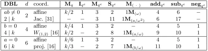
We summarize the operation counts in Table 1. We restrict to even embedding degree and 4 | k for b = 0 as well as to 6 | k for a = 0 because these cases allow using the maximal-degree twists and are likely to be used in practice. We compare the affine counts to costs of the fastest known formulas using projective coordinates taken from [31] and [16]; see these papers for details. For an overview of the most efficient explicit formulas known for elliptic-curve operations see the EFD [10]. We transfer the formulas in [31] to the ate pairing using the trick in [16] where the ate pairing is computed entirely on the twist. In this setting we assume field extensions are constructed in a way that favors the representation of line function values. This means that the twist isomorphism can be different from the one described in this paper. Still, in the cased= 2, evaluation of the line function can not be done inkMq; instead 2 multiplications inFqk/2 need to be done (see [16]). Furthermore, we assume that all precomputations are done as described in the above papers and small multiples are computed by additions.
DBL d coord. Mq Iqe Mqe Sqe M(
·) addqe subqe negqe
ab6= 0
2 affine k/2 1 3 2 1M(ω) 4 6 −
2|k Jac. [31] − − 3 11 1M(a/ω2) 6 17 −
b= 0
4 affine k/4 1 3 2 − 4 5 1
4|k W(1,2)[16] k/2 − 2 8 1M(a/ω) 9 10 1 a= 0
6 affine k/6 1 3 2 − 4 5 1
6|k proj. [16] k/3 − 2 7 1M(b/ω) 11 10 1
Table 1. Operation counts for the doubling step in the ate-like Miller loop omitting 1Sqk+ 1Mqk.
Addition steps in affine coordinates: The line function value has the same shape as for doubling steps. Note that we can replaceR′ byQ′ in the line and compute
lR,Q(P) =yP−α3yQ′−λ(xP −α2xQ′) =yP−αλ′xP+α3(λ′xQ′ −yQ′)
andR′
3=R′+Q′, wherexR′
3=λ ′2−x
R′−xQ′ andyR′
3 =λ
′(xR′−x
R′
3)−yR′. The slope λ′ now is different, namely λ′ = (y
R′ −yQ′)/(xR′ −xQ′). Note that
R′=−Q′ does not occur when computing Miller function values of degree less than r. The cost for doing an addition step is the same as that for a doubling step, except that the cost to compute the slopeλ′ is nowI
qe+Mqe+ 2subqe.
and twist representations and line function evaluation, similar remarks as for doubling steps apply here.
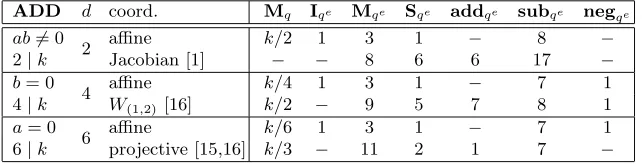
The multiplication withωin the cased= 2 can be done as a precomputation, sinceQ′ is fixed throughout the pairing algorithm. Since other formulas do not have multiplications by constants, we omit this column in Table 2.
ADD d coord. Mq Iqe Mqe Sqe addqe subqe negqe
ab6= 0
2 affine k/2 1 3 1 − 8 −
2|k Jacobian [1] − − 8 6 6 17 −
b= 0
4 affine k/4 1 3 1 − 7 1
4|k W(1,2)[16] k/2 − 9 5 7 8 1
a= 0
6 affine k/6 1 3 1 − 7 1
6|k projective [15,16] k/3 − 11 2 1 7 −
Table 2.Operation counts for the addition step in the ate-like Miller loop omitting 1Mqk.
Affine versus projective: Doubling and addition steps for computing pairings in affine coordinates include one inversion inFqe per step. The various projective
formulas avoid the inversion, but at the cost of doing more of the other opera-tions. How much higher these costs are exactly, depends on the underlying field implementation and the ratio of the costs for squaring to multiplication.
A rough estimate of the counts in Table 2 shows that for Sqe = Mqe or
Sqe = 0.8Mqe (commonly used values in the literature, see [10]), the cost traded
for the inversion in the projective addition formulas is at least 9Mqe. For doubling
steps, it is smaller, but larger than 3Mqe in all cases. Since doubling steps are
much more frequent in the pairing computation (especially when a low Hamming weight for the degree of the used Miller function is chosen), the traded cost in the doubling case is the most relevant to consider.
Example 1. Let ab 6= 0, i.e. d = 2. The cost that has to be weighed against the inversion cost for a doubling step is 9Sqk/2−(k/2)Mq+M(a/ω2)−M(ω)+ 2addqk/2+11sub
qk/2. Clearly, (k/2)Mq <S
qk/2, and we assumeM(ω)≈M(a/ω2) andaddqk/2≈sub
qk/2. IfS
qk/2 ≈0.8M
qk/2, we see that if an inversion costs less than 6.4Mqk/2+ 13add
qk/2, then affine coordinates are better than Jacobian.
In implementations of prime fields, inversions are usually very expensive, i.e. the ratioRq is very large. So the costs for inversions are much higher than the
above-mentioned costs to avoid them. Thus it does not make sense to use affine coordinates. But it is possible to obtain much smaller ratios, e.g. when computing in extension fields. Since the ate pairing requires inversions only inFqe this could
be in favor of affine coordinates. Depending on the specific ratioRq for a given
implementation, affine coordinates might even be faster than projective.
3
Inversions in extension fields for the ate pairing
In this section, we describe and analyze a way to compute inversions in finite field extensions. It is based on a given, fixed implementation of arithmetic in the underlying prime field and explains that the inversion-to-multiplication ratio
R=I/Mdecreases when moving up in a tower of field extensions.
3.1 Inverses in field extensions
The method we suggest for computing the inverse of an element in an extension of some finite fieldFq was originally described by Itoh and Tsujii [32] for binary
fields using normal bases. Kobayashi et al. [34] generalize the technique to large-characteristic fields in polynomial basis and use it for elliptic-curve arithmetic. It is a standard way to compute inverses in optimal extension fields (see [2,27] and [17, Sections 11.3.4 and 11.3.6]).
We requireFqℓ =Fq(α) where αhas minimal polynomial Xℓ−ω for some
ω∈F∗
q and assume gcd(ℓ, q) = 1. Then, the inverse ofβ ∈F∗qℓ can be computed
as
β−1=βv−1 ·β−v,
where v= (qℓ−1)/(q−1) =qℓ−1+
· · ·+q+ 1. Note thatβv is the norm ofβ and thus lies in the base fieldFq. So the cost for computing the inverse ofβ is
the cost for computingβv−1andβv, one inversion in the base fieldF
q to obtain
β−v, and the multiplication ofβv−1 withβ−v. The powers ofβ are obtained by
using theq-power Frobenius automorphism onFℓq.
We give a brief estimate of the cost of the above. A Frobenius computation using a look-up table ofℓ−1 pre-computed values inFqconsisting of powers ofω
costs at mostℓ−1 multiplications inFq (see [34, Section 2.3], note gcd(ℓ, q) = 1).
According to [29, Section 2.4.3] the computation ofβv−1 via an addition chain approach, using a look-up table for each needed power of the Frobenius, costs at most⌊log(ℓ−1)⌋+h(ℓ−1) Frobenius computations and fewer multiplications in Fqℓ. Hereh(m) denotes the Hamming weight of an integerm. Knowing thatβv∈
Fq, its computation fromβv−1 andβ costs at mostℓbase field multiplications,
one multiplication withω, andℓ−1 base field additions. The final multiplication of β−v with βv−1 can be done in ℓ base field multiplications. This leads to an upper bound for the cost of an inversion inFqℓ as follows:
Iqℓ ≤Iq+ (⌊log(ℓ−1)⌋+h(ℓ−1))(Mqℓ+ (ℓ−1)Mq)
LetM(ℓ) be the minimal number of multiplications inFq needed to multiply
two different, non-trivial elements in Fqℓ not lying in a proper subfield of Fqℓ.
Then the following lemma bounds the ratio of inversion to multiplication costs in Fqℓ from above by 1/M(ℓ) times the ratio in Fq plus an explicit constant.
Thus the ratio in the extension improves by roughly a factor ofM(ℓ).
Lemma 1. Let Fq be a finite field, ℓ >1,Fqℓ =Fq(α)withαℓ=ω∈F∗q. Then
using the above inversion algorithm in Fqℓ leads to
Rqℓ ≤Rq/M(ℓ) +C(ℓ),
whereC(ℓ) =⌊log(ℓ−1)⌋+h(ℓ−1) + 1
M(ℓ) 3ℓ+ (ℓ−1)(⌊log(ℓ−1)⌋+h(ℓ−1))
.
Proof. Since M(ℓ) is the minimal number of multiplications in Fq needed for
multiplying two elements in Fqℓ, we can assume that the actual cost for the
latter isMqℓ ≥M(ℓ)Mq. Using inequality (2), we deduce
Rqℓ =Iqℓ/Mqℓ ≤Iq/(M(ℓ)Mq) + ˜C(ℓ) =Rq/M(ℓ) + ˜C(ℓ),
where ˜C(ℓ) =⌊log(ℓ−1)⌋+h(ℓ−1)+(2ℓ+(ℓ−1)(⌊log(ℓ−1)⌋+h(ℓ−1)))/M(ℓ)+ (Mω+ (ℓ−1)addq)/(M(ℓ)Mq). Since M(ω) ≤ Mq and addq ≤ Mq, we get
Mω+ (ℓ−1)addq ≤ℓMq and thus ˜C(ℓ)≤C(ℓ). ⊓⊔
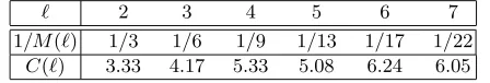
In Table 3 we give values for the factor 1/M(ℓ) and the additive constant C(ℓ) that determine the improvements ofRqℓoverRqfor several small extension
degreesℓ. We take the numbers forM(ℓ) from the formulas given in [38].
ℓ 2 3 4 5 6 7
1/M(ℓ) 1/3 1/6 1/9 1/13 1/17 1/22
C(ℓ) 3.33 4.17 5.33 5.08 6.24 6.05
Table 3.Constants that determine the improvement ofRqℓ overRq
For small-degree extensions, the inversion method can be easily made explicit. We state and analyze it for quadratic and cubic extensions.
Quadratic extensions: Let Fq2 = Fq(α) with α2 = ω ∈ Fq. An element β=b0+b1α6= 0 can be inverted as
1 b0+b1α =
b0−b1α b2
0−b21ω
= b0
b2
0−b21ω − b1 b2
0−b21ω α.
In this case the norm ofβ is given explicitly byb2
0−b21ω∈Fq. The inverse of β
thus can be computed inIq2 =Iq+ 2Mq+ 2Sq+M(ω)+subq+neg
q.
we assume that the cost for a full multiplication in the quadratic extension is at leastMq2 ≥3Mq, i.e. we restrict to the average case where both elements have both of their coefficients different from 0. Thus
Rq2 =Iq2/Mq2 ≤(Iq/3Mq) + 2 =Rq/3 + 2,
where we roughly assume thatIq2 ≤Iq+6Mq. This bound shows that forRq >3 the ratio becomes smaller inFq2. For large ratios inFqit becomes roughlyRq/3.
Cubic extensions: LetFq3 =Fq(α) withα3=ω∈Fq. Similar to the quadratic case we can invertβ=b0+b1α+b2α2∈F∗q3 by
1
b0+b1α+b2α2 = b2
0−ωb1b2 N(β) +
ωb2 2−b0b1 N(β) α+
b2 1−b0b2
N(β) α 2
with N(β) = b3
0+b31ω+b32ω2−3ωb0b1b2. We start by computing ωb1 and ωb2 as well as b2
0 and b21. The terms in the numerators are obtained by a 2-term Karatsuba multiplication and additions and subtractions via 3Mq computing
b0b2, ωb1b2 and (ωb2 +b0)(b2 +b1). The norm can be computed by 3 more multiplications and 2 additions. Thus the cost for the inversion is Iq3 = Iq + 9Mq+ 2Sq+ 2M(ω)+ 4addq+ 4subq. A Karatsuba multiplication can be done
in Mq3 = 6Mq+ 2M(ω)+ 9addq + 6subq. We useMq3 ≥6Mq, assumeIq3 ≤
Iq+ 18Mq and obtain Rq3=Iq3/Mq3 ≤(Iq/6Mq) + 3 =Rq/6 + 3.
Towers of field extensions: Baktir and Sunar [3] introduce optimal tower fields as an alternative for optimal extension fields, where they build a large field extension as a tower of small extensions instead of one big extension. They describe how to use the above inversion technique recursively by passing down the inversion in the tower, finally arriving at the base field. They show that this method is more efficient than computing the inversion in the corresponding large extension with the Itoh-Tsujii inversion directly.
In pairing-based cryptography it is common to use towers of fields to represent the extensionFqk, wherekis the embedding degree. Benger and Scott [9] discuss
how to best choose such towers, but do not address inversions.
3.2 Extension-field inversions for the ate pairing
We have seen in Section 2 that for the ate pairing, the inversions in the doubling and addition steps are inversions in a proper extension field ofFq. We now take
a closer look at specific high-security levels to see which degrees these extension fields have. For a pairing-friendly elliptic curveEoverFq with embedding degree
k with respect to a prime divisor r | #E(Fq), we define the ρ-value of E as
ρ= log(q)/log(r). This value is a measure of the base field size relative to the size of the prime-order subgroup on the curve.
curve subgroup of orderrand in a subgroup of F∗
qk. For efficiency reasons, it is
desirable to balance the security in both groups. The group sizes are linked by the embedding degreek, which leads to desired values forρkas given in Table 4.
security NIST [4] ECRYPT II [43]
(bits) r (bits) qk (bits) ρk qk(bits) ρk
128 256 3072 12 3248 12.69
192 384 7680 20 7936 20.67
256 512 15360 30 15424 30.13
Table 4. NIST [4] and ECRYPT II [43] recommendations for bitsizes of r and qk
providing equivalent levels of security on elliptic-curve point groups and in finite fields.
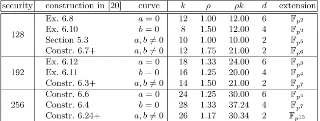
To implement pairings at a given security level, one needs to find a pairing-friendly elliptic curve with parameters of at least the sizes given in Table 4; for efficiency it is even desirable to obtainρkas close to the desired value as possible. An overview of construction methods for pairing-friendly elliptic curves is given in [20]. In Table 5, we list suggestions for curve families by their construction in [20] for high-security levels of 128, 192, and 256 bits. The last column in Table 5 shows the field extensions in which inversions are done to compute the line function slopes. We not only give families of curves with twists of degree 4 and 6, but also more generic families such that the curves only have a twist of degree 2. Of course, in the latter case the extension field, in which inversions for the affine ate pairing need to be computed, is larger than when dealing with higher-degree twists. Because curves with twists of degree 4 and 6 are special (they havej-invariants 1728 and 0), there might be reasons to choose the more generic curves. Note that curves from the given constructions are all defined over prime fields. Therefore we use the notationFp in Table 5.
security construction in [20] curve k ρ ρk d extension
128
Ex. 6.8 a= 0 12 1.00 12.00 6 Fp2 Ex. 6.10 b= 0 8 1.50 12.00 4 Fp2 Section 5.3 a, b6= 0 10 1.00 10.00 2 Fp5 Constr. 6.7+ a, b6= 0 12 1.75 21.00 2 Fp6
192
Ex. 6.12 a= 0 18 1.33 24.00 6 Fp3 Ex. 6.11 b= 0 16 1.25 20.00 4 Fp4 Constr. 6.3+ a, b6= 0 14 1.50 21.00 2 Fp7
256
Constr. 6.6 a= 0 24 1.25 30.00 6 Fp4 Constr. 6.4 b= 0 28 1.33 37.24 4 Fp7 Constr. 6.24+ a, b6= 0 26 1.17 30.34 2 Fp13
Remark 1. The conclusion to underline from the discussion in this section, is that, using the improved inversions in towers of extension fields described here, there are at least two scenarios wheremost implementations of the ate pairing would be more efficient using affine coordinates:
When higher security levels are required, so thatk is large.For example 256-bit security with k = 28, so that most of the computations for the ate pairing take place in the field extension of degree 7, even using a degree-4 twist (second-to-last line of Table 5). In that case, the I/M ratio in the degree-7 extension field would be roughly 22 times less (plus 6) than the ratio in the base field (see the last entry in Table 3). The costs for doubling and addition steps given in the second lines of Tables 1 and 2 for degree-4 twists show that the cost of the inversion avoided in a projective implementation should be compared with roughly 6Sq7 + 5addq7 + 5subq7 extra for a doubling (and an extra 6Mq7 + 4Sq7 + 7addq7 +subq7 for an addition step). In most implementations of the base field arithmetic, the cost of these 16 or 17 operations in the extension field would outweigh the cost of one improved inversion in the extension field. See for example our sample timings for degree-6 extension fields in Table 6 in Section 5. Note there that even the cost for additions and subtractions is not negligible as is usually assumed.
When special high-degree twists are not being used.In this scenario there are two reasons why affine coordinates will be better under most circumstances:
First, the costs for doubling and addition steps given in the first lines of Tables 1 and 2 for degree-2 twists are not nearly as favorable towards projective coordinates as the formulas in the case of higher degree twists. For degree-2 twists, both the doubling and addition steps require roughly at least 9 extra squarings and 13 or 15 extra field extension additions or subtractions for the projective formulas.
Second, the degree of the extension field where the operations take place is larger. See the bottom row for each security level in Table 5, so we have extension degree 6 for 128-bit security up to extension degree 13 for 256-bit security.
4
Sharing inversions for pairing computation
In this section, we revisit a well-known trick for efficiently computing several inverses at once, asymptotically achieving anI/M-ratio of 3. We point out and recall possibilities to improve pairing computation in affine coordinates by using this trick.
4.1 Simultaneous inversions
The inverses ofsfield elementsa1, . . . , ascan be computed simultaneously with
and its inverse (ab)−1. The inverses ofaandbare then found bya−1=b·(ab)−1 andb−1=a·(ab)−1.
In general, for s elements one first computes the products ci = a1· · · · ·ai
for 2 ≤i ≤ s with s−1 multiplications and inverts cs. Then we have a−s1 =
cs−1c−s1. We geta−s−11 by c− 1
s−1 =c−s1as and as−−11 =cs−2c−s−11 and so forth (see [17, Algorithm 11.15]), where we need 2(s−1) more multiplications to get the inverses of all elements.
The cost forsinversions is replaced byI+ 3(s−1)M. LetRavg,sdenote the
ratio of the cost of s inversions to the cost ofs multiplications. It is bounded above by Ravg,s =I/(sM) + 3(s−1)/s≤R/s+ 3, i.e. when the numbers of
elements to be inverted grows, the ratioRavg,s gets closer to 3. Note that most
of the time, this method improves the efficiency of an implementation whenever applicable. However, as discussed in Section 3, in large field extensions, theI/M -ratio might already be less than 3 due to the inversion method from Section 3.1, in which case the sharing trick would make the average ratio worse.
4.2 Sharing inversions in a single pairing computation
Schroeppel and Beaver [40] demonstrate the use of the inversion-sharing trick to speed up a single scalar multiplication on an elliptic curve in affine coordinates. They suggest postponing addition steps in the double-and-add algorithm to ex-ploit the inversion sharing. In order to do that, the double-and-add algorithm must be carried out by going through the binary representation of the scalar from right to left. First, all doublings are carried out and the points that will be used to add up to the final result are stored. When all these points have been collected, several additions can be done at once, sharing the computation of inversions among them.
Miller’s algorithm can also be done from right to left. The doubling steps are computed without doing the addition steps. The required field elements and points are stored in lists and addition steps are done in the end. The algorithm is summarized in Algorithm 2. Unfortunately, addition steps cost much more than in the conventional left-to-right algorithm as it is given in Algorithm 1. In the right-to-left version, each addition step in Line 10 needs a general Fqk
-multiplication and a -multiplication with a line function value. The conventional algorithm only needs a multiplication with a line. These huge costs can not be compensated by using affine coordinates with the inversion-sharing trick.
Algorithm 2Right-to-left version of Miller’s algorithm with postponed addition steps for evenk and ate-like pairings
Input: Q′∈G′
2, P ∈G1, m= (1 =ml−1, ml−2, . . . , m0)2
Output: fm,ψ(Q′)(P) representing a class inF∗qk/(F∗qk)r
1: R′←Q′, f←1, j←0 2: forifrom 0 toℓ−1do 3: if (mi= 1)then
4: AR′[j]←R′, Af[j]←f, j←j+ 1
5: end if 6: f←f2·l
ψ(R′),ψ(R′)(P), R′←[2]R′
7: end for 8: R′←A
R′[0], f←Af[0]
9: for(j←1; j≤h(m)−1;j+ +)do 10: f←f·Af[j]·lψ(R′),ψ(AR′[j])(P), R
′←R′+A
R′[j]
11: end for 12: returnf
cores, once multiple cores can be used with less overhead. It is straightforward to extend this algorithm to more cores.
So we suggest that the parallelized algorithm can be combined with the shared inversion trick when doing the addition steps in the end. The improve-ments achieved by this approach strongly depend on the Hamming weight of the valuemin Miller’s algorithm. If it is large, then savings are large, while for very sparsemthere is almost no improvement. Therefore, when it is not possible to choosem with low Hamming weight, combining the parallelized right-to-left algorithm for pairings with the shared inversion trick can speed-up the compu-tation. Grabher et al. [23] note that when multiple pairings are computed, it is better to parallelize by performing one pairing on each core.
4.3 Multiple pairings and products of pairings
Many protocols involve the computation of multiple pairings or products of pair-ings. For example, multiple pairings need to be computed in the searchable en-cryption scheme of Boneh et al. [13]; and the non-interactive proof systems pro-posed by Groth and Sahai [26] need to check pairing product equations. In these scenarios, we propose sharing inversions when computing pairings with affine coordinates. In the case of products of pairings, this has already been proposed and investigated by Scott [41, Section 4.3] and Granger and Smart [25].
Multiple pairings. Assume we want to computespairings on pointsQ′
iandPi,
i.e. a priori we havesMiller loops to computefm,ψ(Q′
i)(Pi). We carry out these
but rather sliced at the slope denominator inversions. The costs stay the same, except that now the average inversion-to-multiplication cost ratio is 3 +Rqe/s,
wheree=k/danddis the twist degree.
So when computing enough pairings such that the average cost of an inver-sion is small enough, using the sliced-Miller approach with inverinver-sion sharing in affine coordinates is faster than using the projective coordinates explicit formulas described in Section 2.2.
Products of pairings. For computing a product of pairings, more optimiza-tions can be applied, including the above inversion-sharing. Scott [41, Section 4.3] suggests using affine coordinates and sharing the inversions for computing the line function slopes as described above for multiple pairings. Furthermore, since the Miller function of the pairing product is the product of the Miller functions of the single pairings, in each doubling and addition step the line functions can already be multiplied together. In this way, we only need one intermediate vari-ablef and only one squaring per iteration of the product Miller loop. Of course in the end, there is only one final exponentiation on the product of the Miller function values. Granger and Smart [25] show that by using these optimizations the cost for introducing an additional ate pairing to the product can be as low as 13% of the cost of a single ate pairing.
5
Example implementation
The implementation described in this section is an implementation of the optimal ate pairing on a Barreto-Naehrig (BN) curve [8] over a 256-bit prime field, i.e. the curve has a 256-bit prime number n of Fp-rational points and embedding
degreek= 12 with respect ton.
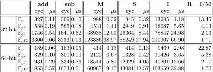
The implementation is part of the Microsoft Research pairing library. It is specialized to the BN curve family but is not specialized for a specific BN curve. It is based on Microsoft Research’s general purpose library for big number arith-metic, which can be compiled under 32-bit or 64-bit Windows. On top of that, we use the tower of field extensions Fp12/Fp6/Fp2/Fp to realize field arithmetic inFp12. In Table 6 we give timings for the required field arithmetic in the fields Fp, Fp2, Fp6, and Fp12 for the bit and 64-bit versions, respectively. The 32-bit timings are for a pure software C-implementation, while the 64-32-bit software makes use of assembly code for base field multiplications, i.e. special code for Montgomery multiplication with a prime modulus of 256 bits, only using the fixed size of the modulus. Note that the timings in cycles and miliseconds stem from two different measurements and thus do not exactly translate.
estimates given there that take into account only multiplications from the base field and neglect all other base field operations.
add sub M S I R=I/M
cyc µs cyc µs cyc µs cyc µs cyc µs
32-bit
Fp 327 0.11 309 0.10 988 0.32 945 0.32 13285 4.18 13.45 Fp2 588 0.19 585 0.18 4531 1.44 2949 0.91 18687 5.65 4.13
Fp6 1746 0.54 1641 0.52 38938 12.09 26364 8.44 78847 24.98 2.03
Fp12 3300 1.06 3233 1.03 123386 38.97 88249 27.94 210907 66.90 1.71
64-bit
Fp 189 0.06 163 0.05 414 0.13 414 0.13 9469 2.98 22.87 Fp2 329 0.10 300 0.10 2122 0.67 1328 0.42 11426 3.65 5.38
Fp6 931 0.29 834 0.26 18544 5.81 12929 4.05 40201 12.66 2.17
Fp12 1855 0.57 1673 0.51 60967 19.17 43081 13.57 103659 32.88 1.70
Table 6. Field arithmetic timings in a 256-bit prime field, on an Intel Core 2 Duo E8500 @ 3.16 GHz under 32-bit/64-bit Windows 7. Average over 1000 operations in cpucycles (cyc) and microseconds (µs).
The pairing implementation uses the usual optimizations. First of all, a twist E′/F
p2 provides the groupG′
2 to represent elements in G2 as described in Sec-tion 2.1. The affine doubling and addiSec-tion steps in Miller’s algorithm are com-puted as shown in Section 2.2. The projective steps use the explicit formulas from the recent paper of Costello et al. [16]. The final exponentiation is done as described in [42], and uses the special squaring formulas given by Granger and Scott [24].
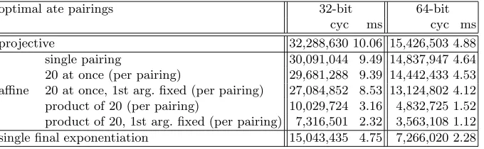
Table 7 gives benchmarking results for several pairing functions in the li-brary, compiled under 32-bit and 64-bit Windows 7, respectively. All functions compute the optimal ate pairing for BN curves as described for example in [39]. The line entitled “20 at once (per pairing)” gives the average timing for one pair-ing out of 20 that have been computed at the same time. This function uses the inversion-sharing trick as described in Section 4.3. The function corresponding to the line “product of 20” computes the product of 20 pairings using the opti-mizations described in Section 4.3. The lines with the attribute “1st arg. fixed” mean functions that compute multiple pairings or a product of pairings, where the first input point is fixed for all pairings, and only the second point varies. In this case, the operations depending only on the first argument are done only once. We list separately the final exponentiation timings. They are included in the pairing timings of the other lines.
Implementation notes.
1. For both the 32-bit and 64-bit versions of the library, a single pairing is com-puted faster with affine coordinates than with projective coordinates. This is due to the relatively lowI/M-ratios in the base fieldFp(13.45 and 22.87
optimal ate pairings 32-bit 64-bit
cyc ms cyc ms
projective 32,288,630 10.06 15,426,503 4.88
single pairing 30,091,044 9.49 14,837,947 4.64 20 at once (per pairing) 29,681,288 9.39 14,442,433 4.53 affine 20 at once, 1st arg. fixed (per pairing) 27,084,852 8.53 13,124,802 4.12 product of 20 (per pairing) 10,029,724 3.16 4,832,725 1.52 product of 20, 1st arg. fixed (per pairing) 7,316,501 2.32 3,563,108 1.12 single final exponentiation 15,043,435 4.75 7,266,020 2.28
Table 7.Optimal ate pairing timings on a 256-bit BN curve, measured on an Intel Core 2 Duo E8500 @ 3.16 GHz under 32-bit/64-bit Windows 7. Average over 20 pairings in cpucycles (cyc) and milliseconds (ms).
the base field combined with the improved inversion for quadratic extensions given in Section 3.1.
2. At this security level (128-bits) and using the special high-degree-6 twist, the projective implementation is almost on par with the affine implementation, so that even a small improvement in the base field multiplication would tip the balance in favor of a projective implementation.
3. However, as was explained in Remark 1 in Section 3.2, either for higher secu-rity levels or for curves without special high degree twists, affine coordinates will be much faster than projective coordinates given our base field and ex-tension field arithmetic. Indeed, our I/M-ratio in a degree 6 extension is already roughly 2, for both our 32-bit and 64-bit versions. With a ratio of 2, projective coordinates are not a good choice.
4. Because ourI/M-ratios in the quadratic field extension are already so close to 3, there is little improvement expected or observed from using the shared inversion tricks discussed in Section 4.
5. Note that field addition and subtraction costs are not negligible, as one might think from the fact that they are not often included in the operation counts when comparing various methods for elliptic curve operations and pairing implementations. In our base field arithmetic, 1 multiplication costs roughly the same as 3 field additions or subtractions, but the relative cost of additions and subtractions in extension fields is significantly less.
6. Note that the ratio of squarings to multiplications changes in the extension fields as well. A squaring in the quadratic extension is done with only 2 multiplications using the fact that the extension is generated by√−1. This improvement carries through to squarings in the higher field extensions.
Comparison to related work. We compare our work with the best results for optimal ate pairing implementations on BN curves that we are aware of.
Recently, there has been significant improvement on pairing implementations for BN curves. The paper [39] presents an implementation that computes the optimal ate pairing on a 256-bit BN curve using one core of an Intel Core 2 Quad in about 4,380,000 cycles. The implementation described in [11] computes the same pairing on a 254-bit BN curve in 2,490,000 cycles on an Intel Core i7.
Software as described in [39] and [11] is much faster than our implementa-tion for the following reason. The above implementaimplementa-tions gain their efficiency by special curve parameter choices combined with a careful instruction scheduling specific to the parameters and certain computer architectures or even proces-sors, in particular resulting in highly efficient multiplications in the base field and the quadratic extension field. Instead, our implementation is based on a general-purpose library for the base field arithmetic which can be compiled on many platforms and works for all BN curves. Thus our implementation is not competitive with specially tailored ones as in [39] and [11]. Nevertheless, the effects implied by the use of affine coordinates that we demonstrated with the help of our implementation also apply to implementations with faster field mul-tiplications. Affine coordinates will then be better only when working with larger extension degrees that occur for higher security levels.
Acknowledgements: We would like to thank Dan Shumow and Tolga Acar for their help with the development environment for our implementation. We thank Steven Galbraith, Diego F. Aranha, and the anonymous referees for their helpful comments to improve the paper.
References
1. Christophe Ar`ene, Tanja Lange, Michael Naehrig, and Christophe Ritzenthaler. Faster computation of the Tate pairing. Journal of Number Theory, 2010. doi:10.1016/j.jnt.2010.05.013.
2. Daniel V. Bailey and Christof Paar. Efficient arithmetic in finite field extensions with application in elliptic curve cryptography. Journal of Cryptology, 14(3):153– 176, 2001.
3. Sel¸cuk Baktir and Berk Sunar. Optimal tower fields. IEEE Transactions on Com-puters, 53(10):1231–1243, 2004.
4. Elaine Barker, William Barker, William Burr, William Polk, and Miles Smid. Recommendation for key management - part 1: General (revised). Technical report, NIST National Institute of Standards and Technology, 2007. Published as NIST Special Publication 800-57,http://csrc.nist.gov/groups/ST/toolkit/ documents/SP800-57Part1_3-8-07.pdf.
5. Paulo S. L. M. Barreto, Steven D. Galbraith, Colm ´O h´Eigeartaigh, and Michael Scott. Efficient pairing computation on supersingular abelian varieties. Designs, Codes and Cryptography, 42(3):239–271, 2007.
6. Paulo S. L. M. Barreto, Hae Yong Kim, Ben Lynn, and Michael Scott. Efficient algorithms for pairing-based cryptosystems. In CRYPTO 2002, volume 2442 of Lecture Notes in Computer Science, pages 354–368. Springer, 2002.
8. Paulo S. L. M. Barreto and Michael Naehrig. Pairing-friendly elliptic curves of prime order. InSelected Areas in Cryptography – SAC 2005, volume 3897 ofLecture Notes in Computer Science, pages 319–331. Springer, 2006.
9. Naomi Benger and Michael Scott. Constructing tower extensions of finite fields for implementation of pairing-based cryptography. In M. Anwar Hasan and Tor Helleseth, editors, Arithmetic of Finite Fields – WAIFI 2010, Istanbul, Turkey, volume 6087 ofLecture Notes in Computer Science, pages 180–195. Springer, 2010. 10. Daniel J. Bernstein and Tanja Lange. Explicit-formulas database. http://www.
hyperelliptic.org/EFD.
11. J.-L. Beuchat, J. E. Gonz´alez D´ıaz, S. Mitsunari, E. Okamoto, F. Rodr´ıguez-Henr´ıquez, and T. Teruya. High-speed software implementation of the optimal ate pairing over Barreto-Naehrig curves. IACR ePrint Archive, report 2010/354, 2010. http://eprint.iacr.org/2010/354.
12. Ian F. Blake, Gadiel Seroussi, and Nigel P. Smart, editors. Advances in Elliptic Curve Cryptography. Cambridge University Press, 2005.
13. Dan Boneh, Giovanni Di Crescenzo, Rafail Ostrovsky, and Giuseppe Persiano. Public key encryption with keyword search. InEUROCRYPT 2004, volume 3027 ofLecture Notes in Computer Science, pages 506–522. Springer, 2004.
14. Henri Cohen, Gerhard Frey, and Christophe Doche, editors. Handbook of Elliptic and Hyperelliptic Curve Cryptography. Chapman and Hall/CRC, 2005.
15. Craig Costello, H¨useyin Hisil, Colin Boyd, Juan Manuel Gonz´alez Nieto, and Ken-neth Koon-Ho Wong. Faster pairings on special Weierstrass curves. In Pairing 2009, volume 5671 ofLecture Notes in Computer Science, pages 89–101. Springer, 2009.
16. Craig Costello, Tanja Lange, and Michael Naehrig. Faster pairing computations on curves with high-degree twists. InPublic-Key Cryptography – PKC 2010, volume 6056 ofLecture Notes in Computer Science, pages 224–242. Springer, 2010. 17. Christophe Doche.Finite Field Arithmetic, chapter 11 in [14], pages 201–237. CRC
press, 2005.
18. Sylvain Duquesne and Gerhard Frey. Background on Pairings, chapter 6 in [14], pages 115–124. CRC press, 2005.
19. Sylvain Duquesne and Gerhard Frey. Implementation of Pairings, chapter 16 in [14], pages 389–404. CRC press, 2005.
20. David Freeman, Michael Scott, and Edlyn Teske. A taxonomy of pairing-friendly elliptic curves. Journal of Cryptology, 23(2):224–280, 2010.
21. Steven D. Galbraith. Pairings, chapter IX in [12], pages 183–213. Cambridge University Press, 2005.
22. Steven D. Galbraith, Keith Harrison, and David Soldera. Implementing the Tate pairing. In Claus Fieker and David R. Kohel, editors, ANTS-V, volume 2369 of Lecture Notes in Computer Science, pages 324–337. Springer, 2002.
23. Philipp Grabher, Johann Großsch¨adl, and Dan Page. On software parallel imple-mentation of cryptographic pairings. InSAC 2008, volume 5381 ofLecture Notes in Computer Science, pages 35–50. Springer, 2009.
24. Robert Granger and Michael Scott. Faster squaring in the cyclotomic group of sixth degree extensions. InPublic-Key Cryptography – PKC 2010, volume 6056 of Lecture Notes in Computer Science, pages 209–223. Springer, 2010.
27. Jorge Guajardo and Christof Paar. Itoh-Tsujii inversion in standard basis and its application in cryptography and codes. Designs, Codes and Cryptography, 25:207– 216, 2001.
28. Darrel Hankerson, Alfred J. Menezes, and Michael Scott. Software implementation of pairings. In Marc Joye and Gregory Neven, editors,Identity-Based Cryptography - Volume 2 Cryptology and Information Security Series. IOS Press, Amsterdam, The Netherlands, The Netherlands, 2008.
29. Darrel Hankerson, Alfred J. Menezes, and Scott Vanstone.Guide to Elliptic Curve Cryptography. Springer New York, Inc., Secaucus, NJ, USA, 2003.
30. Florian Heß, Nigel P. Smart, and Frederik Vercauteren. The eta pairing revisited. IEEE Transactions on Information Theory, 52:4595–4602, 2006.
31. Sorina Ionica and Antoine Joux. Another approach to pairing computation in Edwards coordinates. In Progress in Cryptology – INDOCRYPT 2008, volume 5365 ofLecture Notes in Computer Science, pages 400–413. Springer, 2008. 32. Toshiya Itoh and Shigeo Tsujii. A fast algorithm for computing multiplicative
inverses in GF(2ˆm) using normal bases. Inf. Comput., 78(3):171–177, 1988. 33. Tetsuya Izu and Tsuyoshi Takagi. Efficient computations of the Tate pairing for the
large MOV degrees. InInformation Security and Cryptology - ICISC 2002, Seoul, Korea, November 28-29, 2002, Revised Papers, volume 2587 of Lecture Notes in Computer Science, pages 283–297. Springer-Verlag, 2003.
34. Tetsutaro Kobayashi, Hikaru Morita, Kunio Kobayashi, and Fumitaka Hoshino. Fast elliptic curve algorithm combining Frobenius map and table reference to adapt to higher characteristic. InAdvances in Cryptology - EUROCRYPT 1999, volume 1592 ofLecture Notes in Computer Science, pages 176–189. Springer, 1999. 35. E. Lee, H. S. Lee, and C.-M. Park. Efficient and generalized pairing computation
on Abelian varieties. IEEE Trans. on Information Theory, 55(4):1793–1803, 2009. 36. Victor S. Miller. The Weil pairing and its efficient calculation. Journal of
Cryp-tology, 17(4):235–261, 2004.
37. Peter L. Montgomery. Speeding the Pollard and elliptic curve methods of factor-ization. Mathematics of Computation, 48(177):243–264, 1987.
38. Peter L. Montgomery. Five, six, and seven-term Karatsuba-like formulae. IEEE Transactions on Computers, 54(3):362–369, 2005.
39. Michael Naehrig, Ruben Niederhagen, and Peter Schwabe. New software speed records for cryptographic pairings. In Progress in Cryptology – Latincrypt 2010, volume 6212 ofLecture Notes in Computer Science, pages 109–123. Springer, 2010. Corrected version:http://www.cryptojedi.org/papers/dclxvi-20100714.pdf. 40. Rich Schroeppel and Cheryl Beaver. Accelerating elliptic curve calculations with
the reciprocal sharing trick. Mathematics of Public-Key Cryptography (MPKC), University of Illinois at Chicago, 2003.
41. Michael Scott. Computing the Tate pairing. InCT-RSA, volume 3376 ofLecture Notes in Computer Science, pages 293–304. Springer, 2005.
42. Michael Scott, Naomi Benger, Manuel Charlemagne, Luis J. Dominguez Perez, and Ezekiel J. Kachisa. On the final exponentiation for calculating pairings on ordinary elliptic curves. In Pairing-Based Cryptography – Pairing 2009, volume 5671 ofLecture Notes in Computer Science, pages 78–88. Springer, 2009.
43. Nigel Smart (editor). ECRYPT II yearly report on algorithms and keysizes (2009-2010). Technical report, ECRYPT II – European Network of Excellence in Cryp-tology, EU FP7, ICT-2007-216676, 2010. Published as deliverable D.SPA.13, http://www.ecrypt.eu.org/documents/D.SPA.13.pdf.