Improved Agreeing-Gluing Algorithm
Igor Semaev
Department of Informatics, University of Bergen, Norway [email protected]
Abstract. In this paper we study the asymptotical complexity of solving a system of sparse algebraic equations over finite fields. An equation is called sparse if it depends on a bounded number of variables. Finding efficiently solutions to the system of such equations is an un-derlying hard problem in the cryptanalysis of modern ciphers. New deterministic Improved Agreeing-Gluing Algorithm is introduced. The expected running time of the Algorithm on uniformly random instances of the problem is rigorously estimated. The estimate is at present the best theoretical bound on the complexity of solving average instances of the problem. In particular, this is a significant improvement over those in our earlier papers [20, 21]. In sparse Boolean equations a gap between the present worst case and the average time complexity of the problem has significantly increased. Also we formulateAverage Time Complexity Con-jecture. If proved that will have far-reaching consequences in the field of cryptanalysis and in computing in general.
1
Introduction
1.1 The problem and motivation
Let (q, l, n, m) be a quadruple of natural numbers, where q is a prime power. ThenFq denotes a finite field withqelements andX ={x1, x2, . . . , xn}is a set of variables fromFq. ByXi, 1≤i≤m
we denote subsets ofX of sizeli ≤l. The system of equations
f1(X1) = 0, . . . , fm(Xm) = 0 (1)
is considered, wherefiare polynomials overFqand they only depend on variablesXi. Such equations are calledl-sparse. A solution to (1) overFq is an assignment inFq to variablesX that satisfies all equations (1). That is a vector of lengthnoverFq provided the variablesX are ordered. The main goal is to find all solutions overFq. There may be solutions over the extensions ofFq, but we do not need them. In the most interesting case m=n we will have just one solution overFq on the average.
Deterministic Improved Agreeing-Gluing (IAG) Algorithm which solves the system is here sug-gested. It is presented by two variations. The expected complexity of one variation is rigorously estimated assuming uniform distribution on the problem instances; see Section 1.3. The results provide a significant improvement over earlier average time complexity estimates [20, 21]. Another variation seems require more sophisticated analysis than that presented here.
Anyway, the run-time analysis is more transparent in comparison with that in [20, 21]. It is based on the theory of random allocations [13] as earlier. However, it now requires estimating the probabilities of only few common events; see Section 9. The algorithm running time expectation is the sum of O(n3) terms, each of them is bounded by the same real-valued function in three real
with the advanced optimization package MAPLE [15] in Sections 10 and 11. The computation does not depend onn.
The approach, which exploits the sparsity of equations and doesn’t depend on their algebraic degree, was studied in [28, 17, 20, 21]. These are guess-and-determine algorithms. In sparse equations the number of guesses on a big enough variable subset Y ⊆X and the time to produce them is much lower thanq|Y|due to the Search Algorithm; see Section 8, where the algorithm is described.
This is a more general and efficient method than that in [21]. No preference was previuosly made on which variables to guess. We now argue that guessing values of some particular variables leads to better asymptotic complexity bounds.
The article was motivated by applications in cryptanalysis. Modern ciphers are product ciphers, the mappings they implement are compositions of not so many functions in a low number of vari-ables. The similar is true for underlying one-way functions in asymmetric ciphers. Any one-way function is representable by a low number of small gates as its values should be efficiently com-puted. Intermediate variables are introduced to simplify equations, describing the cipher, and to get a system of sparse equations like (1). More general type of sparse equations called Multiple Right Hand Side linear equations and introduced in [18], is even more convenient tool to write equations from modern ciphers like the AES. An efficient solution to the equations may break the cipher.
Equations common in cryptanalysis depend on large variable sets. Those represented by common dense polynomials are hardly manageable as it is not possible to keep them in computer memory. The equations must be sparse in one or the other sense. For instance, suitable sparsity is low degree polynomials or polynomials that admit only bounded number of terms. In this article we focus on l-sparse equations over finite fields as they are defined by (1). This definition allows more operating freedom and generally results in a more efficient solution than with Gr¨obner basis algorithms. Moreover bounds on the problem average complexity, which is the goal of the present research, are relatively easy to get.
The author is grateful to several anonymous referees at SCC 2010 and ”Mathematics in Com-puter Science” for numerous suggestions on improving the presentation. This is a full paper, the extended abstract is in SCC 2010 [23].
1.2 How to write equations
Let Y be an ordered string of variables and abe anFq-vector of the same length. We say thata is a vector in variables Y, orY-vector, if the entries of amay be assigned to the variablesY, for instance, in case of fixation. We look for the set of all solutions to (1) overFq. Therefore, we only consider forfi polynomials of degree at mostq−1 in each variable.
The main step of the present method is the Search Algorithm; see Section 8. It repeatedly checks whether the systemfi(Xi) = 0, Y =a, for some subsetsY ⊆X andY-vectorsa, has any solution overFq. If there is a solution, then we sayfi(Xi) = 0, Y =aconsistent overFq or simply consistent. One may choose to work with the polynomialsfi(Xi). The decision problem whetherfi(Xi) = 0, Y =ais consistent overFq may then be solved with any Gr¨obner basis algorithm. At least for low q, it may be more convenient in practice to deal with the local solutions Vi overFq. That is the set of Xi-vectors, wherefi is zero. In polynomial algebra terms, Vi are common zeroes of the polynomialsfi(Xi), xq−x, x∈Xi. The setsVi obviously determine all global solutions overFq.
reduced to at mostql+ql−1. . .+q bits per equation with some pre-computation before applying
the Search Algorithm; see Section 8.
1.3 Probabilistic model
Given q, n, m, and l1, . . . , lm ≤ l, uniform distribution on instances is assumed, that is every
instance has the same probability. As any particular information on equations is beforehand as-sumed unknown, this looks the most fair probabilistic model to compute expected complexities. The uniformity is equivalent to
1. the equations in (1) are independently generated. Each equation fi(Xi) = 0 is determined by 2. the subsetXi of sizeli taken uniformly at random from the set of all possible li-subsets ofX,
that is with the probability ln
i
−1,
3. and the polynomialfi taken uniformly at random and independently ofXi from the set of all polynomials of degree≤q−1 in each of variablesXi. In other words, with the equal probability q−qli.
Running time of any deterministic solving algorithm is a random variable under that model. We assume thatm/ntends tod≥1 asq andlare fixed and ntends to infinity.
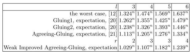
Table 1.Algorithms’ running time:q= 2 andm=n.
l 3 4 5 6
the worst case, [12] 1.324n1.474n1.569n1.637n Gluing1, expectation, [20] 1.262n1.355n1.425n1.479n Gluing2, expectation, [20] 1.238n1.326n1.393n1.446n Agreeing-Gluing, expectation, [21] 1.113n1.205n1.276n1.334n
r 2 3 3 4
Weak Improved Agreeing-Gluing, expectation 1.029n1.107n1.182n1.239n .
2
Previous Ideas
One earlier method [20] is based on subsequent computing solutionsUkto the equation subsystems: f1(X1) = 0, . . . , fk(Xk) = 0 fork= 1, . . . , m. Gluing procedure extends instancesUk to instances Uk+1 by walking throughout a search tree. In the end, all system solutions areUm. The running time is determined by the maximal of|Uk|. Gluing2 is a time-memory trade-off variation of the basis Gluing1 Algorithm. See Table 1 for their running time expectation in case ofnBoolean equations in nvariables and a variety of l. Any instance of (1) may be encoded by a CNF formula with the clause length of at mostk=dlog2qeland indlog2qenBoolean variables; see Section 6. Therefore worst case complexity bounds in [12] for k-SAT are also worst case bounds for equations (1). In Boolean case(q= 2) they are shown in the first line of Table 1.
In Agreeing-Gluing Algorithm [21] we only extend those intermediate solutions from Uk that do not contradict with each of fk+1(Xk+1) = 0, . . . , fm(Xm) = 0. That makes lots of search tree
3
New Approach
The new method has two variations. LetZrdenote variables that occur in at leastrequations (1), andWrdenoteZr-vectors that contradict none of (1). In Weak IAG Algorithm(WIAG), see Section 7, ris a parameter to be chosen to minimize the run-time. The vectors Wr are generated by the Search Algorithm, see Section 8. In case r≥3, the variables Zr are substituted by the entries of a∈Wr. New equations in a smaller variable setX\Zr are encoded by a CNF and deterministic local search algorithm, see Section 6, is applied to find all solutions. Forr= 1, W1are already the
system solutions. Forr= 2, the solutions are easy to generate fromW2; see Lemma 2 below.
This variation is evaluated in Sections 10 and 11 in caseli=l. Two last lines in Table 1 show the expected complexity of the Weak IAG Algorithm and the optimal value ofr. The Agreeing-Gluing Algorithm [21] is a particular case of the present method forr= 1.
In Strong IAG Algorithm(SIAG) the largest r, where Zr is not empty, is taken. The vectors Wr are generated by the Search Algorithm. For eacha∈ Wr the variables Zr are substituted by the entries of a. New l-sparse equations in a smaller variable setX\Zr are to solve. For each of them assignments to Zr−1\Zr that contradict none of the equations are found with the Search
Algorithm. Thus, one recursively computes Wr−1, . . . , W2. All system solutions are then easy to
deduce.
The latter variation should be faster, as the Search algorithm is on the average faster in compar-ison with the local search. However, the estimation of the Strong IAG Algorithm should probably require more sophisticated tools. The work still in progress.
4
Related Methods
Gr¨obner basis algorithm was designed to work with general algebraic equation systems over any ground field; see [4, 14, 10, 11]. It may be used to solving them. The running time is bounded by a value proportional to n+DDωground field operations, where ωis the exponent in matrix multipli-cation complexity. The estimate simplifies to Dnω
for any Boolean equations [3]. The parameter D, called regularity degree, is only computed for semi-regular equations as they are defined in [3]. Theoretical complexity of the Gr¨obner basis algorithms as F4 or F5 on general polynomial equa-tion systems remains unknown. It is also unknown whether an average equaequa-tion system behaves semi-regularly, though this seems plausible [3].
Let l be fixed while n = m tending to infinity. For l-sparse Boolean equation systems each polynomial in (1) admits at most 2l monomials. Then each row in Macaulay matrices has bounded number of nonzero terms. Wiedemann algorithm [26] may likely be used to do the linear algebra step. We then putω= 2. The regularity degree for semi-regular Boolean equations in case n=m was estimated asD=αdn+o(n), whereαd depends on the equations maximal algebraic degreed. So thatα2= 0.09, α3= 0.15, α4= 0.2 and so on; see [2]. By estimating the binomial coefficient, the
complexity is then 22H(αd)n up to a polynomial factor, whereH(α) is the binary entropy function.
One can see that only for quadratic semi-regular polynomials the running time is lower than 2n, brute force complexity, and equal to 1.832n bit operations. By computing the exact value of the regularity degree, the conjectural running time still exceeds the brute force complexity forn= 200; see [1]. The best heuristic bound is of order 1.724n [27], where the method was combined with variable guessing.
even in non-quadratic case; see Table 1. Table 2 presents extended data. It shows cl for a larger variety of l, where the expected complexity, computed at r= 2, on Boolean l-sparse equations is cn
l . That compares favorably with the above estimates by Gr¨obner basis algorithms for quadratic sparse polynomials at least forl≤19.
Table 2.IAG Algorithm(r= 2) base constantcl,q= 2 andm=n.
l 3 4 5 6 7 8 9 10 11 12 13 14 15 16 17 18 19
cl1.029 1.118 1.191 1.252 1.304 1.347 1.385 1.418 1.448 1.474 1.497 1.518 1.538 1.555 1.571 1.586 1.600
Sparse equations may be encoded by a CNF formula and solved with a SAT-solving software. The asymptotical complexity of modern SAT-solvers, as MiniSat [9], is unknown, though they may be fast in practice [7, 25] for relatively low parameters.
5
Notation, Basic Lemma and Example
LetY ⊆X be a subset of variables. The following statement is the basement for the IAG Algorithm complexity analysis in Section 10.
Lemma 1. Let W be the set ofY-vectors consistent with each equation (1). Let X1, X2, . . . , Xm
be fixed and polynomials f1, f2, . . . , fm be taken uniformly at random as in Section 1.3. Then the
expectation of |W| is given by
Ef1,...,fm|W|=q |Y|
m Y i=1
1−(1−1
q) q|Xi\Y|
.
Proof. Let a be a Y-vector. We compute Pr(a ∈ W), the probability that fi(Xi) = 0, Y = a is consistent for alli. As fi are independent,
Pr(a∈W) = m Y i=1
Pr(fi(Xi) = 0, Y =aconsistent).
Upon fixationY =a, the polynomialfi(Xi) produces a uniformly random polynomial in variables Xi\Y. It follows from Lemma 4 that
Pr(fi(Xi) = 0, Y =aconsistent) = 1−(1−1
q) q|Xi\Y|
and this value doesn’t depend on a. So
Ef1,...,fm|W|=
X a
Pr(a∈W) =q|Y|Pr(a∈W) =q|Y| m Y i=1
1−(1−1
q) q|Xi\Y|
.
According to Section 1.3,X1, X2, . . . , Xmare random subsets inX. Therefore the full
expecta-tion of|W|is given by
E|W|=EX1,...,Xm(Ef1,...,fm|W|) =EX1,...,Xm q |Y|
m Y i=1
1−(1−1
q) q|Xi\Y|
!
(2)
by Lemma 5 below. The setY may depend on the subsetsX1, X2, . . . , Xmand therefore be random.
LetZr(k) be the set of variables that appear in at least r ofX1, . . . , Xk and letWr(k) beZr(k
)-vectors consistent with each equationfi(Xi) = 0. We have Zr(r)⊆Zr(r+ 1)⊆. . .⊆Zr(m) =Zr. The Search Algorithm extends instancesWr(k) to Wr(k+ 1), where the output is Wr =Wr(m). From (2)
E|Wr(k)|=EX1,...,Xm q |Zr(k)|
m Y i=1
1−(1−1
q)
q|Xi\Zr(k)|
!
. (3)
The maximal of these expectations upper bounds the complexity of first stage of the WIAG Al-gorithm up to a polynomial factor. It is estimated in Section 10. The second stage complexity for r≥3 is similarly estimated in Section 11. Three cases should be studied separately.
Case r= 1. ThenUm=W1, all system solutions in variablesX1∪. . .∪Xm. ExtendingW1(k) to
W1(k+ 1) by walking over a search tree is the Agreeing-Gluing Algorithm [21].
Case r= 2. Remark that variables in differentXi\Z2 are pairwise different. So everya∈W2 is
extendable to at least one solution of (1). Moreover the following statement holds.
Lemma 2. Let Xi1, Xi2, . . . , Xis be all variable sets such thatXij *Z2. After reordering of
vari-ables it holds that
Um= [ a∈W2
{a} ×Vi1(a)×Vi2(a). . .×Vis(a), (4)
whereVi(a)are all projections toXi\Z2 of theFq-solutions tofi(Xi) = 0, Z2=a.
Example.Let the system of three Boolean equations be given with their local solutions:
x1x2x3
0 0 1 1 0 0 1 1 1 1 0 1 ,
x3x4x5
0 0 0 1 0 1 1 1 1 0 0 1 ,
x5x6x7
0 0 0 0 1 1 1 1 0 1 0 1 .
We see Z2(2) = {x3} and W2(2) = {0,1}, so Z2(3) = {x3, x5} and W2(3) = {00,01,11}. The
directed products (4) are:
x3x5x1x2 x4 x6x7
0 0 1 0 × 0 × 0 0 1 1 0 1 1 0 × 0 × 1 0 0 1 1 1 0 0 × 0 × 1 0
1 1 1 0 1
1 0
.
Case r≥3. The Search Algorithm returns some a∈Wr. The variablesZr are substituted by the entries ofa. The problem is represented by ak-CNF withk=dlog2qeland inn1=dlog2qe |X\Zr|
Boolean variables. Local search algorithm, described in [8], is used to find all solutions. In worst case, that takes O((N + 1)(2− 2
k+1)
n1) bit operations up to a polynomial factor to find all N
solutions; see Section 6.
6
k-CNF and Local Search
Conjunctive normal form(CNF for short) is a conjunction of disjunctions asx(c1)
i1 ∨. . .∨x
(ck)
ik called
clauses, wherex(0)=xandx(1) = ¯x. The disjunction termsxand ¯xare called literals. If the length
of each clause in a CNF is at mostk, then it is calledk-CNF. Letq= 2, andf(x1, . . . , xl) = 0 be
any Boolean equation inl Boolean variables. Let
(a11, . . . , a1l), . . . ,(as1, . . . , asl)
be all binary strings such thatf(ai1, . . . , ail) = 1.
Lemma 3. Binary string (b1, . . . , bl)is a solution to f(x1, . . . , xl) = 0 iff it is a satisfying assign-ment for the CNF
Ff = (x(a11)
1 ∨. . .∨x (a1l)
l )∧. . .∧(x
(as1)
1 ∨. . .∨x (asl)
l ).
If all equations (1) are Boolean, one constructsl-CNF inn variables asF =V
iFfi. Binary string
(b1, . . . , bn) is a solution to (1) iff it is a satisfying assignment forF.
Generally, elementsa∈Fq may be encoded with the numbers 0, . . . , q−1. Every variable xin Fq is written withr=dlog2qeBoolean variablesyr−1, . . . , y0, such thatx=aiff (yr−1, . . . , y0) =
(br−1, . . . , b0), wherebi ∈ {0,1} anda=br−12r−1+. . .+b0. So Fq-solutions to f(x1, . . . , xl) = 0 are written as binarylr-strings.
As in Lemma 3, for the set of binarylr-strings complimentary to those solutions one constructs a k-CNF in k = lr variables. We do that for each equation in (1). Resulting k-CNF in n1 = nr
variables is a conjunction of them. Solving (1) is equivalent to finding satisfying assignments to that CNF and therefore is NP-hard as it is polynomially equivalent to ak-SAT problem.
Local search is designed to solve satisfiability problems; see [16, 19]. Given ak-CNF inn vari-ables, guess an initial assignment to all variables. Repeat 3ntimes: if the formula is satisfied, then terminate; let there be some clause not being satisfied by the current assignment, then pick one of its literals uniformly at random and flip its value in the current assignment. The probability of finding a satisfying assignment is at least 23(2(kk−1))n; see [19], and the expected number of this
procedure repetitions before the satisfying assignment if found is (2−2
k)
nup to a polynomial factor.
A deterministic version is described in [8]. Within poly(n)(2− 2
k+1)
n operations the algorithm
finds a satisfying assignments or returns the CNF is unsatisfiable. Therefore local search may be used to compute allN solutions in time at most (N+ 1)(2− 2
k+1)
n up to a polynomial factor.
7
Weak IAG Algorithm
root at level 0 is labeled by∅. Vertices at levelk≥rare labeled by∅ ifZr(k) =∅ and by vectors Wr(k) if this set is not empty. If Wr(k) =∅, then there is no any vertices at levelk, so the whole system of equations is inconsistent.
Let a ∈ Wr(k) be a level k vertex label. It is connected to a level k+ 1 vertex labeled by b∈Wr(k+ 1) wheneverais a sub-vector ofb. Remark thatZr(k)⊆Zr(k+ 1).
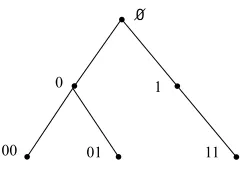
The search tree for the example system is presented in Fig. 1, wherer= 2. Level 2 vertices are labeled byW2(2) ={0,1}, vectors in variablesZ2(2) ={x3}. The vertices at level 3 are labeled by
W2(3) ={00,01,11}, vectors in variablesZ2(3) ={x3, x5}. We now describe the Algorithm. More
formal description of its first stage is in the next Section.
Stage 1( Search Algorithm) It starts at the root. Let the Algorithm be at a level k vertex labeleda. If k= 0, then we extendato all possible Zr(r)-vectors. Ifk≥r, then we extenda toZr(k+ 1)-vectors by trying all possible assignments to variablesZr(k+ 1)\Zr(k).
Letb be one such extension. If Zr(k+ 1) =b(or Zr(r) =b if k= 0) is consistent with every equation in (1), then b ∈ Wr(k+ 1). Return b if k+ 1 = m. The Algorithm walks to the vertex labeledb. Otherwise, another assignment is taken to extenda. If all the assignments are exhausted andk= 0, then stop. Ifk >0, then the Algorithm backtracks to the levelk−1. This stage output isWr=Wr(m). If no vertex at levelm is hit , then the system has no solution.
Stage 2 Let the Algorithm achieve a vertex at level m labeled bya ∈Wr. If r= 1, then a is a system solution. Ifr= 2, then the system solutions are deduced with (4). If r ≥3, a system of l-sparse equations in variables X \Zr after substituting Zr by constants a is solved with deterministic local search; see Section 6.
0 1
00 01 11
∅
Fig. 1.The search tree.
Remark that instead of all possible assignments to variablesZr(k+ 1)\Zr(k) one may only take the projections of local solutions fk+1(Xk+1) = 0 to those variables. That slightly accelerates the
first stage.
Theorem 1. Let N be the number of the system solutions.
2. The complexity of the second stage is at most (N +|Wr|) cn−|Zr| bit operations up to a
polynomial factor, where c = (2− 2
ldlog2qe+1)
dlog2qe. If r≥3, then the Algorithm run-time is the
sum of its stages complexities.
Proof. The complexity of the first stage is
mq|Zr(r)|+m
m−1
X k=r
|Wr(k)|q|Zr(k+1)\Zr(k)|
decisions whetherfi(Xi) = 0, Y =bis consistent for someY. The latter costsO(1) bit operations. Because|Zr(r)|and|Zr(k+ 1)\Zr(k)|are at mostl, the first statement is then true.
Leta∈WrandNabe the number of the system solutions after the variablesZrbeing substituted by the entries of a. The complexity of the second stage is
X a∈Wr
(Na+ 1)cn−|Zr|= (N+|Wr|)cn−|Zr|
bit operations up to a polynomial factor. That implies the second statement. ut
We realize thatEN =qn−m as E
f1,...,fmN =q
n−m for any fixed variable sets Xi. Under the
probabilistic model the values|Wr(k)|are random. The expected complexity of the first stage(and of the whole algorithm forr= 1,2) is proportional tom+m2max
kE|Wr(k)|,where E|Wr(k)| is represented by (3) and estimated in Section 10. For the second stage complexity we have
E(N+|Wr|)cn−|Zr|=Eqn−mcn−|Zr|+E|Wr|cn−|Zr|.
The expectations ofqn−mcn−|Zr|and|Wr|cn−|Zr|are estimated in Section 11, where the latter may
be shown dominates the sum.
For a range of r the estimates are computed with an optimization software like MAPLE; see [15]. One then finds r to minimize the running time expectation. Remark that the computation does not depend onn.
8
General Search Algorithm
Given Y ⊆X, this general Algorithm finds allY-vectors overFq that consistent with each of (1). A subset sequenceY1⊆Y2⊆. . .⊆Ys=Y is taken. That defines a search tree. The root is labeled
by∅, the vertices at levels 1≤k≤s are labeled byYk-vectors that do not contradict any of (1). We denote themW(k). Verticesaandbat subsequent levels are connected ifais a sub-vector ofb. The algorithm walks with backtracking throughout the tree by constructing instancesW(k). There are q|Yk+1\Yk| extensions to any ofW(k). Each of them should be checked for consistency withm
equations. We represent the Algorithm with a pseudocode. Let, by agreement,Y0=∅andY0-vector
a=∅ is consistent with every equation (1). The extension toa=∅ with an assignmentc to some variables isc.
Procedure EXTEND(k, a).
input:0≤k≤s−1 and aYk-vectoraconsistent with each of (1).
1. for every assignment to variablesYk+1\Yk do
2. extendato aYk+1-vectorb. Letb be consistent with every equation in (1). Ifk+ 1< s, then
call recursively EXTEND(k+1,b). Ifk+ 1 =s, then returnb. Ifb is inconsistent with at least one equation, then take another assignment.
3. If all assignment are exhausted andk= 0, then stop. Ifk >1, then return.
The Search Algorithm is EXTEND(0,∅) and its running time is proportional to
m(q|Y1|+|W(1)|q|Y2\Y1|+|W(2)|q|Y3\Y2|+. . .+|W(s−1)|q|Ys\Ys−1|)
operations. A sequence of subsets that minimizes the running time may be taken. How to do that is generally an interesting open problem. In IAG Algorithms the sequence is Zr(r)⊆Zr(r+ 1)⊆ . . .⊆Zr(m) =Zr.
To save time and memory, one may solve the decision problems in advance and keep the tracks. For each equation one keeps the decision( 1 or 0) on whetherfi(Xi) = 0, Xi∩Yk =ais consistent, where a has q|Xi∩Yk| possible values and k = 1, . . . , s. As there are at most l different Xi∩Yk,
then that requires at mostql+ql−1+. . .+qbits of memory. It is not necessary to keep any local
solutions.
In practice, one may want to find weather a Yk-vectoracontradicts the whole system (1) but not only each of the equations taken separately. One then runs the Agreeing Algorithm [18, 24] after the variables Yk get substituted by constants a. Even if no contradiction is found, one may learn values of some new variables. That improves the method efficiency. However such a variation seems difficult to evaluate.
9
Tools
In this Section we collect miscellaneous auxiliary statements.
Let H be the set of all polynomials over Fq in l ≥ 1 variables, whose degree in each of its variables is at most q−1. LetH1 be the subset of polynomialsf ∈H, where the equationf = 0
has no solutions overFq.
Lemma 4. Every polynomial f ∈ H defines a mapping f : Fl
q → Fq and vice versa. That is a one-to-one correspondence. So|H|=qql
and|H1|= (q−1)q
l
.
Proof. The number of polynomials inH and the number of mappingsFl
q →Fq isqq
l
. One proves if a polynomial f ∈ H defines an identically zero mapping, then all its coefficients are 0. Really, f(x1, x2, . . . , xl) =fq−1x
q−1
1 +. . .+f1x1+f0, wherefi are polynomials of degree at mostq−1 in each ofx2, . . . , xl, they are constants ifl= 1. Let f be 0 onFql. After fixation ofx2, . . . , xl by any constants inFq, we get a polynomial inx1which is 0 onFq. Therefore, its coefficients are zeros as,
otherwise, it can not have more thanq−1 different roots. That proves the statement forl= 1. If l >1, then for the same reason the polynomialsfi are 0 on Fl−1
q and by induction they all have zero coefficients. We concludef has zero coefficients.
Iff1, f2 ∈ H define the same mapping, then f1−f2 defines an identically zero mapping and,
therefore,f1=f2. That proves the above correspondence is one-to-one. The polynomials fromH1
correspond to the mappings without zero-values. Their number is (q−1)ql
. ut
Lemma 5. [21] For the full expectation ofη=η(x, y)we have
Ex,yη=Ex(Ey(η)).
Random Allocations Theory studies random allocations of particles(balls, shots) into boxes, see [13]. Letkcomplexes of particles be independently and uniformly allocated inton≤1 boxes,li≤n particles at the i-th allocation. This means that at the i-th allocation any li boxes are occupied with the equal probability ln
i
−1. This is how variable sets X
1, . . . , Xm are generated according
to Section 1.3. We will need to upper bound the probability of several events defined by such allocations. There is some useful theory in [13] developed mostly for allocations of particles one after the other, that is by complexes of size 1. The following Lemma relates the probability of the same event under the two types of allocation.
Letν1, . . . , νn be the string of box frequencies, that isνi is the number of particles in the i-th
box. Let A = A(ν1, . . . , νn) be any event depending on νi. Let also Pr(A| l1, . . . , lk) denote the
probability of the eventAunder the allocation by complexes ofl1, . . . , lk particles.
Lemma 6.
Pr(A|l1, . . . , lk)≤
Pr(A|1, . . . ,1) Qk
i=1(1−1/n). . .(1−(li−1)/n)
,
wherePr(A|1, . . . ,1)is the probability ofAunderL=l1+. . .+lk particles are allocated one after
the other.
Proof. LetLparticles be independently and uniformly allocated intonboxes one after the other. Let Bdenote the event that the firstl1particles were allocated into different boxes, the followingl2were
allocated into different boxes and etc, until the lastlk particles were allocated into different boxes. In other words, the eventB occurs if the particles are allocated by complexes of sizel1, l2, . . . , lk. ThenPr(B) =Qki=1(1−1/n). . .(1−(li−1)/n) as the particles were allocated independently. By the complete probability formula we get
Pr(A|1, . . . ,1) =Pr(B)Pr(A|B) +Pr( ¯B)Pr(A|B¯)
≥Pr(B)Pr(A|B) =Pr(B)Pr(A|l1, . . . , lk)
as Pr(A|B) =Pr(A|l1, . . . , lk). That proves the Lemma. ut
Let f(z) = P∞ k=0akz
k, where real ak ≥ 0, be a non-zero analytic function. We denote fn(z) = P∞
k=0an,kz
k for any naturaln.
Lemma 7. 1.For any realz >0
an,k ≤f
n(z)
zk =e
nlnf(z)−klnz. (5)
2.Let ai, aj >0for somei6=j. Then at any realz >0 the derivative of zf0(z)
f(z) is positive.
Proof. The expansion offn has only nonnegative coefficients, soa
n,kzk≤fn(z). That proves the first statement. To prove the second statement one represents
zf0
f 0
=zf
00f−zf02+f0f
f2 =
P∞ l=0blzl
f2 ,
where bu = Puk=0(u−k+ 1)(u−2k+ 1)akau−k+1 = P
bu+1 2 c
k=0 (u−2k+ 1)2akau−k+1. Therefore
To minimize the bound (5) one may take a positive root z0 to (nlnf(z)−k lnz)0 = 0 or,
equivalently,
nzf
0(z)
f(z) =k.
if there exist any. In case there is only one root, the Lemma estimate is proportional to the main term of the asymptotic expansion foran,kwith the saddle point method asnandktend to infinity; see [5]. Lemma 7 estimate is then asymptotically close to the real value ofan,k. We use rather (5) than the saddle point method in Lemmas 8, 9 and 13.
Let µr = µr(t, n) be the number of boxes with just r particle after uniform allocation of t particles into nboxes one after the other. Letµ0
r(l1, . . . , lk, n) be the number of boxes with justr particle after uniform allocation ofkcomplexes byl1, . . . , lkparticles intonboxes. The probability of some events related toµ0ris required in what follows. We here estimate the probability of them for the allocation of particles one after the other, that is in case of variables µr. Then Lemma 6 is used in Section 10.
LetE(xµr1
1 . . . x
µrs
s ) be the expectation of the random variablex
µr
1
1 . . . x
µrs
s , wherex1, . . . , xs
are any variables. By definition,
E(xµr1
1 . . . x
µrs
s ) = X k1,...,ks
Pr(µr
1 =k1, . . . ,µrs =ks)x
k1
1 . . . x
ks
s .
Theorem 2 in Chapter 2, Section 1 of [13] states
∞
X t=0
ntzt t! E(x
µr
1
1 . . . x
µrs
s ) =
ez+z r1
r1!
(x1−1) +. . .+
zrs
rs!
(xs−1) n
. (6)
In particular, we get
∞
X t=0
ntzt t! E(x
µ0
0 . . . x
µr−1
r−1 ) =
ez+ (x0−1) +. . .+
zr−1
(r−1)!(xr−1−1) n
.
We there put x0=. . .=xr−1= 0 and get
ez−1−z . . .− z
r−1
(r−1)! n
=
∞
X t=nr
ntzt
t! Pr(µ0= 0, . . . ,µr−1= 0)
as Pr(µ0= 0, . . . ,µr−1= 0) = 0 fort < nr. Letg(x) =ex−1−x . . .− xr−1
(r−1)!.
Lemma 8. Let r≥1. For any natural numbert≥nr
Pr(µ0(t, n) = 0, . . . ,µr−1(t, n) = 0)≤ g
n(x)t!
xtnt ,
wherexis the only nonnegative root of the equation
nxg
0(x)
Proof. We have g(x) = xrr! +(xrr+1)!+1 +. . .. So xgg(0x(x)) tends to r as x→ 0+. Also it tends to ∞as
x→ ∞. By Lemma 7, the derivative of xgg(0x(x)) is positive at positivex. Therefore, the equation (7) has just one nonnegative root fort≥nr.
Fort > nr the statement is true by Lemma 7. Let t=nr, then the root x= 0. One sees that gn(x)t!
xtnt is defined atx→0
+ and equal to (nr)!
(r!)nnnr. One directly computes
Pr(µ0(nr, n) = 0, . . . ,µr−1(nr, n) = 0) = (nr)! (r!)nnnr.
The statement is true for anyt≥nr. That proves the Lemma. ut
Letr≥2. It follows from (6) that
∞
X t=0
ntzt t! E(x
µ1
1 . . . x
µr−1
r−1 ) =
ez+z(x1−1) +. . .+
zr−1
(r−1)!(xr−1−1) n
. (8)
Substitutexi=xi fori= 1, . . . , r−1. Then
∞
X t=0
ntzt t! E(x
µ1+2µ2+...+(r−1)µr−1
)
=
ez−
z+. . .+ z r−1
(r−1)!
+
zx+. . .+(zx) r−1
(r−1)! n
.
By the definition of expectation,
E(xµ1+2µ2+...+(r−1)µr−1) =
t X k=0
xkPr(µ1+ 2µ2+. . .+ (r−1)µr−1=k)
because Pr(µ1+ 2µ2+. . .+ (r−1)µr−1=k) = 0 if k > t. We denotezxbyxand get from the
last two identities that
X t≥k
ntzt−kxk
t! Pr(µ1+ 2µ2+. . .+ (r−1)µr−1=k)
=
ez−
z+. . .+ z r−1
(r−1)!
+
x+. . .+ x r−1
(r−1)! n
,
where the left hand side sum is overt andksuch thatt≥k≥0. We now putz= 0 and get
1 +x+. . .+ x r−1
(r−1)! n
=
(r−1)n X t=0
ntxt
t! Pr(µ1+ 2µ2+. . .+ (r−1)µr−1=t).
We remark that the probability is zero ift >(r−1)n. Leth(y) = 1 +y . . .+(yrr−−1)!1 .
Lemma 9. Let r≥2. For any integer numbert such that 0≤t≤(r−1)nwe have
Pr(µ1+ 2µ2+. . .+ (r−1)µr−1=t)≤h
n(y)
wherey is the only nonnegative root (including∞) of the equation
nyh
0(y)
h(y) =t. (9)
Proof. yhh(0(yy)) tends to 0 asy →0+. Also it tends tor−1 asy→ ∞. By Lemma 7, the derivative
of yhh(0y(y)) is positive at positive y. Therefore, the equation (9) has just one nonnegative root for 0≤t≤(r−1)nincludingy= 0 fort= 0 andy=∞fort= (r−1)n.
Let 0< t <(r−1)n. The equation (9) has the only positive root. The estimate is true by the first statement of Lemma 7. Lett= 0, theny = 0 and the Lemma is true as both the sides of the inequality are 1. Let t= (r−1)n, theny=∞. The right hand side of the inequality is defined at y=∞and equal to ((r−1)!)t! nnt. By direct calculation,
Pr(µ1+ 2µ2+. . .+ (r−1)µr−1=t) =Pr(µr−1(t, n) =n) = t! ((r−1)!)nnt.
That proves the Lemma. ut
From the Stirling approximation tok!, see [6], we get
Lemma 10. For every integer numberk≥0 it holds that
kke−k ≤k!≤kke−kp2π(k+ 1).
10
Complexity Estimate. Stage 1
Let r ≥2 and li = l for alli = 1, . . . , m. We now estimate the expectation of |Wr(k)| with (3). Its maximum in k will be estimated with (17). According to the probabilistic model, X1, . . . , Xm are uniformly allocated into the whole variable setX of sizen. So we use the language of particle allocation into nboxes from now. In particular, Zr(k) is the set of boxes with at leastr particles after uniform allocation bykcomplexes of size l. We split the product in (3):
E|Wr(k)|=EX1,...,Xm
q|Zr(k)|
k Y i=1
1−(1−1
q)
q|Xi\Zr(k)|
m Y j=k+1
1−(1−1
q)
q|Xj\Zr(k)|
.
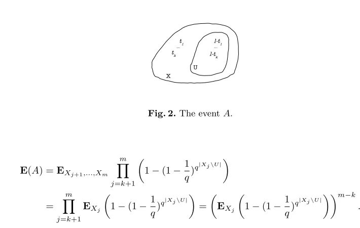
We say the eventA=A(U, t1, . . . , tk) occurs ifZr(k) =U and|Xi\U|=ti, wherei= 1, . . . , k; see
Fig. 2. With the conditional expectation formula we get
E|Wr(k)|= X
U X t1,...,tk
q|U| k Y i=1
1−(1−1
q) qti
E(A)Pr(A), (10)
whereU runs over all subsets ofX and 0≤ti ≤l and we denoted
E(A) =EX1,...,Xm
m Y j=k+1
1−(1−1
q)
q|Xj\Zr(k)|
X U l-t1 ... l-tk t1 ... tk
Fig. 2.The eventA.
So
E(A) =EXj+1,...,Xm
m Y j=k+1
1−(1−1
q) q|Xj\U|
= m Y j=k+1
EXj
1−(1−1
q) q|Xj\U|
=
EXj
1−(1−1
q) q|Xj\U|
m−k .
We remark thatE(A) only depends on the sizeuof the setU, and not on the set itself. Letu=βn, where 0≤β≤1, then
EXj(1−(1−
1 q)
q|Xj\U|) = 1− l X t=0
u l−t
n−u t n l (1− 1 q)
qt = 1− l X t=0
βn l−t
n−βn t n l (1− 1 q)
qt.
By taking limn→∞, we get
Lemma 11. Asntends to ∞
EXj(1−(1−
1 q)
q|Xj\U|) =F(β) +O(1 n),
whereF(β) = 1−Plt=0 l t
βl−t(1−β)t(1−1
q)
qt andO(1
n) is uniformly bounded inβ.
Lemma 11 impliesE(A)≤(F(β) +)m−k,whereis any positive number andnis big enough. LetL=lk=αn, where 0≤α≤dl. So m−k
n = m
n − α
l. As m
n tends tod, then
E(A)≤(F(β) +)(d−αl)n (11)
for any positiveand for all big enoughn. We now estimate the probability of the eventA. Let as above |U|=u.
Lemma 12. LetL=lk andT =t1+. . .+tk. Then
Pr(A)≤
u n
L−T n−u n
T
P1(L−T, u)P2(T, n−u)
Qk i=1
l ti
Ql−1
i=1(1−
i n)
k ,
where
P1(L−T, u) =Pr(µ0(L−T, u) = 0, . . . ,µr−1(L−T, u) = 0),
Proof. Letu= 0, thenT =LandAoccurs if in the allocation ofX1, . . . , Xk every variable is hit
at mostr−1 times. So by Lemma 6,
Pr(A)≤Ql−P12(L, n)
i=1(1−
i n)k
,
and the statement is true. Let u=n, thenT = 0 andAoccurs if in the allocation of X1, . . . , Xk
every variable is hit at leastrtimes. So by Lemma 6,
Pr(A)≤Ql−P11(L, n)
i=1(1−
i n)k
,
and the statement is true. So we can assume 0< u < n. We say the eventB occurs if|Xi\U|=ti fori= 1, . . . , k. ThenPr(A) =Pr(B)Pr(A|B).
Pr(B) = k Y i=1
Pr(|Xi\U|=ti) = k Y i=1
u l−ti
n−u ti n l = = k Y i=1 l ti u n
l−tin−u
n
ti (1−1
u). . .(1− l−ti−1
u )(1−
1
n−u). . .(1− ti−1
n−u) (1− 1
n). . .(1− l−1
n )
= u n
L−T n−u n T Qk i=1 l ti Qk i=1(1−
1
u). . .(1− l−ti−1
u ) Qk
i=1(1− 1
n−u). . .(1− ti−1
n−u) Ql−1
i=1(1−
i n)
k .
The event A|B occurs if and only if the following two events A1 and A2 occur simultaneously.
First, the complexes ofl−t1, . . . , l−tk particles are allocated into|U|=uboxes, where each box
is occupied by at leastr particles. Second, the complexes of t1, . . . , tk particles are allocated into
|X\U|=n−uboxes, where each box is occupied by at mostr−1 particles; see Fig. 2. These are independent events. ThereforePr(A|B) =Pr(A1)Pr(A2).
The eventA1occurs if and only ifµ0i(l−t1, . . . , l−tk, u) = 0 fori= 0, . . . , r−1. The eventA2
occurs if and only if µ0i(t1, . . . , tk, n−u) = 0 fori≥r. The latter is equivalent to
µ01(t1, . . . , tk, n−u) + 2µ02(t1, . . . , tk, n−u) +. . .+ (r−1)µ0r−1(t1, . . . , tk, n−u) =T.
See the definition ofµ0sin Section 9. By Lemma 6,
Pr(A1)≤
P1(L−T, u)
Qk i=1(1−
1
u). . .(1− l−ti−1
u )
and
Pr(A2)≤
P2(T, n−u)
Qk i=1(1−
1
n−u). . .(1− ti−1
n−u)
SoPr(A) =Pr(B)Pr(A|B) =
=Pr(B)Pr(A1)Pr(A2)≤
u n
L−T n−u n
T
P1(L−T, u)P2(T, n−u)
Qk i=1
l ti
Ql−1
i=1(1−
i n)k
.
From (10), asE(A) only depends onu, andPr(A) only depends onu, t1, . . . , tk we get
E|Wr(k)|= n X u=0 n u
quE(A) X t1,...,tk
k Y i=1
1−(1−1
q) qti
Pr(A). (12)
From (12) by Lemma 12,
E|Wr(k)| ≤ Ql−1 1
i=1(1−
i n) k n X u=0 n u
quE(A) (13)
× L X T=0 CT u n
L−Tn−u n
T
P1(L−T, u)P2(T, n−u),
where
CT = X t1+...+tk=T
k Y i=1 l ti
1−(1−1
q) qti
.
Let
f(z) = l X t=0
l
t 1−(1− 1 q)
qt
zt.
It is obvious thatfk(z) =Plk
T=0 CT zT.
Lemma 13. For every 0 ≤ T ≤ l k we have CT ≤ fkz(Tz), where z is the only nonnegative
root(including ∞forT =lk) to the equation kzff(0z(z))=T.
Proof. It is similar to the proofs of Lemmas 8 and 9. ut
LetT =γn, where 0≤γ≤α. By Lemma 8,P1(L−T, u)≤
gu(x) (L−T)!
xL−T uL−T , wherexis a nonnegative
root of the equationβxgg(0x(x)) =α−γ. Therefore, by estimating (L−T)! with Lemma 10, we get
P1(L−T, u)≤
" gβ(x) xα−γ
α−γ βe α−γ + #n , (14)
for any positive and big enoughn. By Lemma 9,P2(T, n−u)≤ h
n−u(y)T!
yT (n−u)T.Therefore,
P2(T, n−u)≤
h1−β(y) yγ
γ (1−β)e
γ +
n
, (15)
for any positiveand all bign, wherey is a nonnegative root to (1−β)yhh(0y(y)) =γ. By Lemma 13,
CT ≤
fαl(z) zγ
n
wherez is a nonnegative root to αlzff(0(zz)) =γ. We remark that for any positivebounds (11), (14), (15) are true simultaneously for anyα, β, γ and big enoughn. Therefore, taking all these bounds into account, from (13) we get
E|Wr(k)| ≤ (Qln+ 1)(−1 lm+ 1)
i=1(1−
i n)m
max
max
qβgβ(x)h1−β(y)fα
l(z) (α−γ)α−γ γγ
ββ(1−β)1−βxα−γ yγ zγ eα F(β) d−α
l
+
n ,
for any positive and big enough n, where Lemma 10 was used to bound the binomial coefficient n
u
. Therefore,
E|Wr(k)| ≤(maxG(α, β, γ) +)n (17)
for any positive and big enoughn, where
G(α, β, γ) = q
βgβ(x)h1−β(y)fα
l(z) (α−γ)α−γγγ
ββ(1−β)1−β xα−γ yγ zγ eα F(β) d−α
l.
The maximum in (17) is over 0 ≤β ≤1 and 0 ≤γ ≤α. We remark that the parameters α, β, γ should satisfyrβ≤α−γ and (r−1)(1−β)≤γ, otherwiseP1(L−T, u) = 0 orP2(T, n−u) = 0.
The first stage complexity is upper bounded by (17) with the maximum over above α, β, γ, where nonnegativex, y, z satisfy
βxg
0(x)
g(x) =α−γ, (18)
(1−β)yh
0(y)
h(y) =γ, (19)
α l
zf0(z)
f(z) =γ. (20)
However, the function G(α, β, γ) may have some singularities. For instance, at β = 0, we should have α−γ= 0 and every 0≤x≤ ∞is the solution to (18). The similar is true atβ= 1 with (19) and atα= 0 with (20). So one may then take a small1>0 and consider the extrema ofG(α, β, γ)
in the area 1≤β ≤1−1,1≤α≤dl, where the function is well-defined and continuous. Out of
this area the contribution of the right hand side terms in (13) is negligible. The maximum is unique and it is computed with an advanced optimization package like MAPLE.
11
Complexity Estimate. Stage 2
We recall that if r ≤ 2, then nothing to do. Let r ≥ 3. Let Wr = Wr(m) and Zr = Zr(m). Let X1, . . . , Xm be fixed and f1, . . . , fm randomly generated. It was proved in Section 7 that the expected complexity of the second stage isE(qn−m+|W
r|)cn−|Zr|, wherec is defined in Theorem 1. As in (3), we prove
E|Wr|cn−|Zr|
=EX1,...,Xm q
|Zr|cn−|Zr|
m Y i=1
1−(1−1
q)
q|Xi\Zr|
LetL=lm. Similarly to (13),
E|Wr|cn−|Zr|
≤ Ql−1 1
i=1(1−
i n) m n X u=0 n u
qucn−u
×
L X T=0
CT u n
L−Tn−u n
T
P1(L−T, u)P2(T, n−u),
whereCT =Pt1+...+tm=T
Qm i=1
l ti
1−(1−1
q)
qti. Therefore,
E|Wr|cn−|Zr|
≤
maxc1−βG(dl, β, γ) +n
, (21)
for any positive and big enough n. The maximum is over 0 ≤ β ≤ 1 and 0 ≤ γ ≤ dl, where nonnegativex, y, zsatisfy (18),(19),(20) andα=dl. Similarly to (13),
Eqn−mcn−|Zr|≤ Ql−1 1
i=1(1−
i n) m n X u=0 n u
qn−mcn−u
×
L X T=0
CT0 u
n
L−Tn−u n
T
P1(L−T, u)P2(T, n−u),
whereCT0 =P
t1+...+tm=T
Qm i=1
l ti
= lmT. Therefore,
Eqn−mcn−|Zr|≤
max
q1−dc1−βgβ(x)h1−β(y) (dl)dl ββ(1−β)1−β xdl−γyγ edl
+
n
(22)
for any positive and big enough n. The maximum is over 0 ≤ β ≤ 1 and 0 ≤ γ ≤ dl, where nonnegative x, y satisfy (18),(19). Computations with MAPLE, similar to those in the previous Section, shows that E|Wr| cn−|Zr| dominates the complexity of the second stage and the overall algorithm complexity is dominated by the first stage at least for the parameters in Tables 1 and 2.
12
Trivially Unsolvable Equations
Trivially unsolvable equations are often generated according to the Section 1.3 model. However that phenomenon only negligibly contributes to the average complexity bounds if they are exponential. The probability that a randomly chosen equation inl variables is solvable overFq, i.e., admits at least one solution overFq, is 1−(1−1
q) ql
. So the probability the equation system (1) is trivially
unsolvable( at least one of the equations has no solutions over Fq) is 1− h
1−(1−1
q) qlim
. This
value tends to 1 asl andqare fixed andm=dntends to infinity. It is very easy to recognize, with some average complexityR, a trivially unsolvable equation system. However, for smalldthat only gives a negligible contribution to the average complexity estimate while it is exponential. Really, letQdenote average complexity of a deterministic algorithm on all instances of (1). LetQ1 denote
each equation has at least one solution overFq. In both cases uniform distribution is assumed. By the conditional expectation formula,
Q=
1−(1−1
q) ql
dn
Q1+ 1−
1−(1−1
q) ql
dn! R.
Therefore, Q1 <
h
1−(1−1
q)
qli−dnQ. For q = 2 and d= 1 that will only change the bound at l= 3. For the Weak IAG Algorithm,Q1becomes bounded by 1.033n whileQis bounded by 1.029n
for largen. For all otherl the influence is negligible: estimates forQandQ1 are almost identical.
For larger d= 1 +δ the contribution is larger, but Qbecomes sub-exponential fast, that follows from the analysis in Sections 10 and 11. SoQ1remains bounded by a very low exponential function
at least for lowδ. In fact, we believe thatQ1becomes sub-exponential too, though it is not proved
here.
Generally, a subsystem of somet ≥2 equations may be inconsistent(without solutions). Then the whole system is inconsistent too. At least for low t the case may be identified by trying mt possible t-subsystems and therefore in polynomial time providing m does not grow very fast. It seems difficult to compute the probability of the event and give its asymptotical analysis. Fort= 2 some heuristic argument shows that slightly affects algorithm’s average running time only forq= 2 and very low l as it is exponential. That is despite the probability presumably tends to 1 as for t= 1. Anyway, the algorithms studied here equally handle this and more complicated cases.
13
Average Time Complexity Conjecture
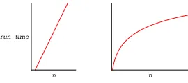
A drastic improvement over last few years in average time complexity of solving (1) raises the question about the function type that may represent it. Exponential function in n representing the run-time of an Algorithm is, by definition, (1 +)n, where is a positive constant. For any sub-exponential function we have positive=(n)→0 asntends to infinity. We remark
Fig. 3.Typical exponential and sub-exponential functions in log-scale
1. forq= 2 and very low las 3,4 the estimates presented in Table 1 are as (1 +)n, wherehas tendency to diminish to 0,
2. generally, aslis bounded andngrows, the same type function(exponential or sub-exponential) likely represents the problem complexity for low and largerl,
Therefore, the following statement called Average Time Complexity Conjecture might be true(it was already formulated in [22]).
There exists an algorithm whose expected time complexity on uniformly random instances (1)is sub-exponential innasq andl are fixed, m≥nwhilentends to infinity.
Symmetric ciphers security is based on the assumption of exponential complexity. A cipher is commonly considered broken if there is an attack whose running time is less than the full search of the key-space, no matter how small the gain is. That differs much from the asymmetric case, where there are effective methods of sub-exponential complexity for integer factoring and discrete logarithms in finite fields. In elliptic curve crypto the underlying problem is exponential, though only half of the key-space in logarithmic measure is to be searched. The similar is true for lattice based crypto-systems.
We believe that sparse equation systems over finite fields are of fundamental importance in cryptanalysis as they provide a tool to write computational problems from either symmetric or asymmetric ciphers in one way. From the point of view of the above conjecture and precedent discussion, it would not be a big surprise if those problems are in nature sub-exponential. Remark that does not contradict with the problem of solving sparse polynomial equations over finite fields is still NP-hard.
Finding the conjectural algorithm(that may be already a Sat-solver like MiniSat, but we do not have any proof of that) might imply a series of improvements from the crypto communities as it was with the index calculus for discrete logs and factoring. Therefore, if proved the conjecture may have far-reaching consequences in the field of cryptanalysis, as changing the symmetric ciphers security assumption or may be breaking some of them, and in computing in general. Its publication may stimulate research in the field.
Previously, for quadratic semi-regular Boolean equation systems it was shown the Gr¨obner basis algorithm is of sub-exponential complexity providedn=o(m); see [2]. The present conjecture claims that is true for average sparse equation systems regardless their regularity and algebraic degree, and for anym≥n.
References
1. C. Bouillaguet, H.-C. K. Chen, C.-M. Cheng, T. Chou, R. Niederhagen, A. Shamir, and B.-Y. Yang,Fast exhaustive search for polynomial systems inF2, IACR ePrint Archive, report 2010/313.
2. M. Bardet, J.-C.Faug´ere, and B. Salvy,Complexity of Gr¨obner basis computation for semi-regular overde-termined sequences overF2 with solutions inF2,Research report RR–5049, INRIA, 2003.
3. M. Bardet, J-C. Faug´ere, B. Salvy and B-Y. Yang,Asymptotic Behaviour of the Degree of Regularity of Semi-Regular Polynomial Systems, in MEGA 2005, 15 pages.
4. B. Buchberger,Theoretical Basis for the Reduction of Polynomials to Canonical Forms,SIGSAM Bull. 39(1976), 19-24.
5. E.T. Copson,Asymptotic expansions,Cambridge University Press, 1965.
6. R. Courant,Differential and integral calculus, vol. 1,Interscience publishers, 1988.
7. N. T. Courtois and G. V. Bard,Algebraic Cryptanalysis of the Data Encryption Standard, in Cryptogr. and Coding, LNCS 4887, pp. 152-169, Springer-Verlag, 2007.
8. E. Dantsin, A. Goerdt, E. A. Hirsch, R. Kannan, J. M. Kleinberg, C. H. Papadimitriou, P. Raghavan, U. Schning,A deterministic(2−2/(k+ 1))nalgorithm fork-SAT based on local search.Theor. Comput. Sci. 289(2002), pp.69–83.
10. J.-C. Faug`ere,A new efficient algorithm for computing Grbner bases (F4),Journal of Pure and Applied Algebra, vol. 139 (1999), pp. 61-88.
11. J.-C. Faug`ere,A new efficient algorithm for computing Gr¨obner bases without reduction to zero (F5), in ISSAC 2002, pp. 75 – 83, ACM Press, 2002.
12. K. Iwama,Worst-Case Upper Bounds for kSAT,The Bulletin of the EATCS, vol. 82(2004), pp. 61–71. 13. V. Kolchin, A. Sevast’yanov, and V. Chistyakov,Random allocations,John Wiley & Sons, 1978. 14. D. Lazard, Gr¨obner-bases, Gaussian elimination and resolution of systems of algebraic equations, in
EUROCAL 1983, pp. 146–156.
15. MAPLE home page, http://www.maplesoft.com
16. C. H. Papadimitriou. On selecting a satisfying truth assignment, In Proc. FOCS’91, pages 163–169, 1991.
17. H. Raddum,Solving non-linear sparse equation systems overGF(2)using graphs,University of Bergen, preprint, 2004.
18. H. Raddum, I. Semaev, Solving Multiple Right Hand Sides linear equations, Des. Codes Cryptogr., vol.49 (2008), pp.147–160.
19. U. Sch¨oning,A probabilistic algorithm for k-Sat based on limited local search and restart,Algoritmica, 32(2002), 615-623
20. I. Semaev,On solving sparse algebraic equations over finite fields, Des. Codes Cryptogr., vol. 49 (2008), pp.47–60.
21. I. Semaev,Sparse algebraic equations over finite fields,SIAM J. on Comp., vol. 39(2009), pp. 388–409. 22. I. Semaev and M. Mikus,Methods to solve algebraic equations in cryptanalysis,Tatra Mountains Math.
Publ.,45(2010), 107-136.
23. I. Semaev, Improved Agreeing-Gluing Algorithm, 2nd Int. Conf. on Symb. Comp. and Crypt., Royal Holloway, University of London, UK, June 23-25, 2010,(2010), 73-88.
24. I. Semaev, Sparse Boolean equations and circuit lattices, Des. Codes Cryptogr., vol. 59 (2011), pp. 349–364.
25. T.E.Schilling and H.Raddum Solving Equation Systems by Agreeing and Learning, in WAIFI 2010, LNCS 6087, pp. 151-165,Springer-Verlag, 2010.
26. D. H. Wiedemann,Solving sparse linear equations over finite fields,IEEE Trans. Information Theory, vol. 32(1986), pp. 54–62.
27. B.-Y. Yang, J-M. Chen, and N.Courtois, On asymptotic security estimates in XL and Gr¨obner bases-related algebraic cryptanalysis,LNCS 3269, pp. 401–413, Springer-Verlag, 2004.