Use of Coefficient of Variation in Assessing Variability of Quantitative Assays

Use of Coefficient of Variation in Assessing Variability of

Quantitative Assays

George F. Reed,

_{* Freyja Lynn,}

_{and Bruce D. Meade}

National Eye Institute, National Institutes of Health, Bethesda,1_{and Center for Biologics Evaluation}

and Research, Food and Drug Administration, Rockville,2_Maryland

Received 26 March 2002/Returned for modification 19 June 2002/Accepted 22 August 2002

We have derived the mathematical relationship between the coefficient of variation associated with repeated measurements from quantitative assays and the expected fraction of pairs of those measurements that differ by at least some given factor, i.e., the expected frequency of disparate results that are due to assay variability rather than true differences. Knowledge of this frequency helps determine what magnitudes of differences can be expected by chance alone when the particular coefficient of variation is in effect. This frequency is an operational index of variability in the sense that it indicates the probability of observing a particular disparity between two measurements under the assumption that they measure the same quantity. Thus the frequency or probability becomes the basis for assessing if an assay is sufficiently precise. This assessment also provides a standard for determining if two assay results for the same subject, separated by an intervention such as vaccination or infection, differ by more than expected from the variation of the assay, thus indicating an intervention effect. Data from an international collaborative study are used to illustrate the application of this proposed interpretation of the coefficient of variation, and they also provide support for the assumptions used in the mathematical derivation.

Although assay variability is well recognized as pertinent to the interpretation of quantitative bioassays such as the en-zyme-linked immunosorbent assay (ELISA), few tools that link assay precision with interpretation of results are readily avail-able. In our investigations, we have expanded on previous studies that evaluated the relationship between assay precision and the capabilities and limitations of a given assay system. In this article we develop a simple procedure to determine the probability that an assay will accurately discern whether two samples have the same analyte concentration or not based on a knowledge of the assay variability as measured by the coef-ficient of variation (CV).

In many laboratories, the variability of the ELISA and other methods of chemical assay that produce continuous-type val-ues is summarized not by the standard deviation (SD) but by the CV, which is defined as the SD divided by the mean, with the result often reported as a percentage. The main appeal of the CV is that the SDs of such assays generally increase or decrease proportionally as the mean increases or decreases, so that division by the mean removes it as a factor in the variabil-ity. The CV is therefore a standardization of the SD that allows comparison of variability estimates regardless of the magni-tude of analyte concentration, at least throughout most of the working range of the assay.

In serological assays a twofold difference in measurements of the same sample has been widely regarded as the upper limit on acceptable variability, and the frequency of such differences among pairs of repeated measurements has been proposed as an apt index for assay variability (5). Wood (4) showed the

mathematical relationship between that frequency and the size of the SD of repeated assay measurements, under the assump-tion that the logarithm of measurements is normally distrib-uted. The tables he provided indicate how small an SD of the log measurements must be in order to ensure that only some predetermined fraction of pairs of measurements differ by a factor of two or more. Wood’s formulation was a valuable link between the precision of titration assays and an operational assessment of assay performance.

As expressed above, in the context of serum assays and other applications the CV may be preferred over SD as a measure of precision, but there is no published formulation that links the CV to assay performance in a manner analogous to Wood’s treatment of the SD in the log scale. Such a formulation would be even more useful if it were to generalize from twofold to k-fold disparities in replicate measurements (wherekcan be any number greater than one and arbitrarily close to one). This generalization would take advantage of the fact that ELISAs and other assays with continuous scales are capable of mea-suring a continuous range of differences in samples, unlike classic titration assays utilizing step-wise, usually twofold, serial dilutions. The intent of this article is to introduce the mathe-matical relationship between the CV and the frequency of k-fold or more-disparate assay values when the same sample is subjected to repeated measurements. We also demonstrate how this relationship can be used to address practical problems in a clinical laboratory.

MATERIALS AND METHODS

The probability that two independent measurements from the same sample

will differ by a factor ofkor more is derived in Appendix A under the assumption

that assay values are lognormally distributed, i.e., that they are normally distrib-uted after a logarithmic transformation. This assumption is supported by the fact that calibration and resultant measurement errors usually take place in a loga-rithmic scale (1). The derived formula is the basis for the construction of a

* Corresponding author. Mailing address: National Eye Institute, 31 Center Dr., MSC-2510, Building 31, Room 6A52, Bethesda, MD 20892-2510. Phone: (301) 496-1331. Fax: (301) 496-2297. E-mail: gfr @nei.nih.gov.

1235

on August 17, 2020 by guest

http://cvi.asm.org/

Downloaded from

on August 17, 2020 by guest

http://cvi.asm.org/

Downloaded from

on August 17, 2020 by guest

http://cvi.asm.org/

nomogram that plots the probabilities for a range of values of CV andk. A partial estimation, by Monte Carlo simulation methods, of the distribution of the

number of twofold disparate pairs amongnreplicates is undertaken in Appendix

B. The resulting table (see Table 2) is proposed for use in monitoring the quality and consistency of the laboratory assay process. Use of the formula and Table 2 is illustrated by their application to data from an international collaborative study

of ELISA methods to quantify human serum antibodies againstBordetella

per-tussisantigens (3). In that study assays on 21 serum samples were performed by 33 laboratories. For the purpose of comparing levels of assay precision among laboratories, each laboratory conducted 15 repeated measurements on each sample, and these measurements were the basis for the CV estimates and vari-ability assessments made in this article. The large number of replicates per sample in the study enabled an additional use of these data: to compare the

actual number ofk-fold disparate pairs with the number predicted by the derived

formula. Computation and graphs were accomplished with Statistical Analysis System (SAS Institute, Cary, N.C.) and S-Plus (Insightful Corporation, Cam-bridge, Mass.) software.

RESULTS

For a specified value of the CV for a given assay the prob-ability that two replicate measurements differ by a factorkor more is given by equation A4 of Appendix A, restated here:

p共k兲⫽2⌽

冋

_冑

e(CV2⫹1)

册

For example, the frequency of replicates that differ by 10% or more (so thatk⫽1.1) from an ELISA with a CV of 15% is calculated as

p(1.1)⫽2⌽

再

_冑

e[(15/100)2⫹1]

冎

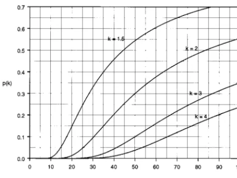
Alternatively, p(k) for kvalues of 1.5, 2, 3, and 4 may be obtained from the nomogram of Fig. 1, which graphs the prob-ability on curves specific to these values ofk.

Equation A5 of Appendix A gives the CV that is associated with a specified frequency, and this value may also be approx-imated by inspection of the nomogram. Obtaining values of the CV this way may be helpful as an exercise to view how the CV corresponds to some hypothetically varied values ofkandp(k), but note that, in clinical laboratory settings, it may not be

possible to dramatically reduce the assay variability, i.e., the CV, by manipulation of assay conditions, apart from radical changes in assay materials and procedures. Due to this prac-tical immutability, the CV will usually serve as a given quantity, and equation A4 will usually be the relevant formula for re-lating CV,k, andp(k).

Equation A4 allows for the restatement of the CV in a metric, p(k), that bears an operational meaning familiar to researchers investigating infectious disease pathology and im-munology. In some vaccine clinical trials, for example, the fraction of trial participants whose serum antibody concentra-tions increase by more than twofold from baseline after vacci-nation may be taken as an indicator of the vaccine’s immuno-genicity and a surrogate of its efficacy. The choice of a twofold increase (which is equivalent to a difference of 0.301 in the log10scale) is a convention that reflects the belief that a lesser

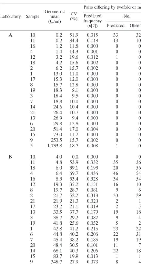
change is probably due not to an actual increase in concentra-tion but to random error. Knowledge of the CV of the assay under these conditions and application of the formula permit calculation of the likelihood of random twofold increases. The belief in the rarity of twofold increases may now be subject to verification. As an example, we refer to the assays quantifying antibodies against pertactin from one of the laboratories, lab-oratory A, that participated in the international collaborative ELISA study. As seen in Table 1, of the 21 serum samples, this laboratory measured 19 with a CV under 20%. The Table 1 results are presented in order of the geometric mean concen-trations of the samples and so reveal that the two CVs that exceed 20% are associated with low levels of analyte, which approached the method’s limit of detection. The high CVs at these levels demonstrate the expected loss of precision when quantifying samples at the extreme ends of the assay’s range. We generalize, then, that the CV in the working range for this laboratory will not exceed 20%. By application of the formula, we determine that for an assay with a CV of 20% there will be 1.3% random twofold changes, half of which will be increases. Thus, in a trial of 200 participants with baseline and postvac-cination pertactin levels assayed by laboratory A, no more than one or two participants will be expected to have a twofold increase, if there is no vaccine effect on antibody levels. The null hypothesis of that trial would be that the portion of two-fold increases does not exceed 0.7%. On the other hand, if the assay were less precise, say with a CV of 30%, the expected number of twofold random increases would be about 10. The null hypothesis would be that the percentage of twofold in-creases does not exceedp(2)/2 or 4.7%. Knowledge of the CV and its interpretation through p(k) is in this way helpful in setting the null hypothesis for vaccine clinical trials or other seroconversion studies to account for random outcomes not related to the intervention under investigation.

A second benefit of linking the CV and the frequency of k-fold disparate pairs is the ability to monitor a laboratory’s performance with respect to what is expected according to its assumed CV. If a laboratory has established that it performs a certain assay with known precision and if random error is the only anticipated source of difference in assays, such as among replicate measurements of the same sample, then too many k-fold differences in pairs of measurements would signal the presence of outliers or some divergence from the assay proce-dure with which the CV is associated. The definition of “too

FIG. 1. Nomogram for relating the CV to the probability that two assay measurements from the same analyte sample will differ by a factorkor more.

on August 17, 2020 by guest

http://cvi.asm.org/

many” may be arbitrarily set, and for our purposes we define “too many differences,” consistent with the hypothesis testing convention, as any number of differences that occur with a tail probability of 0.05 or less. Table 2 displays estimates of the upper 5% tails of the distribution of the number of twofold disparate pairs amongnreplicates (n⫽2,. . ., 15) for various assumed values of CV. This table was constructed, as detailed in Appendix B, from a very large number of simulations of lognormally distributed assay values and is applicable to any lognormal data regardless of mean, variance, or measurement units. The entries are critical values, and observations that exceed them constitute statistical evidence that the actual CV may be higher than assumed. To illustrate the use of Table 2, we refer again to laboratory A. It is established that its per-tactin assay CV should not exceed 20%. In a subsequent run of 10 replicates on a sample, there are 45 ways to make pairs. Suppose that six of those pairs differed by at least twofold.

From Table 2, for a CV of 20% and ann of 10, the critical value is 4, and the occurrence of 6 alerts the observer that some factor may have interfered with the normal conduct of the assay.

The high number of replicates produced by the laboratories in the collaborative study presented the opportunity to discern how well the derivedp(k) fits actual data. For this demonstra-tion, data from laboratory B (Table 1) were included with those from laboratory A. Laboratory B was selected to contrast with A since it displayed more difficulty with the samples in terms of variability. All but one CV exceeded 20%, and the estimated percentage of twofold disparate pairs associated with the CVs was greater than 10% for more than one-half of the samples. (Sample 10 is excluded from consideration in the last sentence because all of its measurements were below the limit of detection and, by the analysis protocol, they were assigned a value of one-half the limit. Since they all then had the same value, the SD and CV were both zero. A CV of zero is an indicator of assay limitation and not a true measure of variability.)

For the 15 replicates per sample there were 105 possible pairings, and the predicted number of k-fold disparate pairs among them is 105䡠p(k). The data from the two selected laboratories were examined to determine the number of pairs that differed by a factor k of 2 or more, and the predicted numbers of such pairs were calculated (Table 1). Herep(k) is not known exactly because it is based on the CV, which must be estimated from the data, so that the predicted number itself is subject to some random variation. Nevertheless, for both lab-oratories there was good correspondence between predicted and observed frequencies for the vast majority of samples. The exceptions are, from Laboratory B, samples 16 and 18, which fall in the lower range of amount of analyte. The high level of agreement between observed and predicted numbers offers some validation of the use of equation A4 and of the lognor-mality assumption upon which it is based.

DISCUSSION

The development of the relationship between the CV and p(k), the probability ofk-fold or more differences in two assays

TABLE 1. Variability summary

Laboratory Sample Geometricmean

(U/ml) CV (%)

Pairs differing by twofold or more Predicted

frequency

(p[2])

No.

Predicted Observed

A 10 0.2 51.9 0.315 33 32

11 0.2 34.4 0.143 13 10

16 1.2 11.8 0.000 0 0

4 1.4 14.3 0.001 0 0

12 3.2 19.6 0.012 1 0

18 4.2 15.6 0.002 0 0

2 6.2 15.7 0.002 0 0

1 13.0 11.0 0.000 0 0

17 15.3 12.0 0.000 0 0

8 15.7 12.8 0.000 0 0

19 18.3 8.1 0.000 0 0

3 18.4 9.5 0.000 0 0

7 18.8 10.0 0.000 0 0

14 24.6 10.4 0.000 0 0

21 26.4 10.7 0.000 0 0

13 26.9 9.4 0.000 0 0

6 29.8 12.8 0.000 0 0

20 51.4 17.0 0.004 0 0

15 73.0 11.2 0.000 0 0

9 253.5 15.7 0.002 0 0

5 1,133.8 18.7 0.008 1 0

B 10 4.0 0.0 0.000 0 0

11 4.8 53.9 0.332 35 36

18 6.0 39.1 0.193 20 56

4 6.4 69.7 0.436 46 54

16 8.3 53.4 0.328 34 54

12 19.3 35.2 0.151 16 10

8 19.7 28.7 0.081 9 6

2 21.7 52.2 0.318 33 29

21 21.9 21.3 0.020 2 1

17 23.2 21.1 0.019 2 5

13 33.5 37.7 0.179 19 18

3 38.7 29.2 0.087 9 4

19 41.8 25.6 0.052 5 2

1 42.8 41.2 0.215 23 22

6 44.8 40.2 0.206 22 31

7 45.4 38.2 0.185 19 19

20 48.4 30.5 0.101 11 7

14 68.1 40.3 0.206 22 18

15 83.7 19.9 0.013 1 1

9 348.7 27.9 0.073 8 4

5 1,450.9 21.9 0.023 2 2

TABLE 2. 5% Critical values for number of twofold disparate pairs

No. of

replicates No. ofpairs

5% critical valuea_{for a CV (%) of:}

14 16 18 20 22 24 26 28 30 35 40 45 50

2 1 1 1 1 1 1 1

3 3 1 1 1 1 2 2 2 2 3 3 3 3 3

4 6 1 1 1 2 2 3 3 3 4 4 4 5 5

5 10 1 1 1 2 3 3 4 4 5 5 6 7 7

6 15 1 1 2 2 3 4 5 5 6 7 8 9 10

7 21 1 1 2 3 4 5 6 6 7 9 11 12 13

8 28 1 1 2 3 4 6 7 8 9 11 13 15 16

9 36 1 2 3 4 5 7 8 9 10 13 16 18 19

10 45 1 2 3 4 6 7 9 11 12 16 19 21 24

11 55 1 2 3 5 7 9 11 12 14 19 22 25 28 12 66 1 2 3 5 7 10 12 14 16 21 26 30 33 13 78 1 2 4 6 8 11 13 16 19 25 30 34 38 14 91 1 2 4 6 9 12 15 18 21 28 34 39 43 15 105 1 3 4 7 10 13 17 20 23 31 38 44 49

a_{If the number of observed pairs equals or exceeds the table value, the null}

hypothesis that the CV is at most the indicated value is rejected.

on August 17, 2020 by guest

http://cvi.asm.org/

of the same sample, enhances the usefulness in clinical labo-ratory work of the CV, which has two advantages over the SD. First, as noted earlier, the CV is dimensionless and therefore does not vary with changes in measurement units. In a similar fashion,p(k) is the same regardless of the base of the logarithm by which the original values are transformed; equation A4, which uses the natural logarithm, is universally applicable. Thus, if other statistical analysis requires a logarithm, chosen for convenience or even arbitrarily, other than the natural logarithm, p(k) is unaffected and always calculated the same way. This property of invariance contrasts with the probabilis-tic interpretation of the SD, which differs with choice of loga-rithm base. Second, although equation A4 is predicated on the assumption that assay values are lognormally distributed, the CV is the ratio of the SD to the mean of the original values, and correspondinglyp(k) refers to ratios of the original values. Thus the interpretation of variability is always in terms of original values. On the other hand, Wood’s system, founded on the SD, requires the SD to be calculated from the transformed assay values and is dependent on which logarithm base is used. We have presented two important applications of the for-mulation that links CV andp(k): (i) to assess whether or not the difference between two paired measurements is due to random variation and (ii) to assess whether the variation in a set of replicates is larger than that implied by the assumed CV. For both applications the starting point is the assumption of values forkand CV. For the first applicationp(k) denotes how likely it is that two assay values from samples with the same analyte concentration will differ by the factorkor more. Ap(k) of 0.05, for example, suggests that such a difference is suffi-ciently infrequent when the concentrations are equal that its occurrence provides support for the conclusion that the con-centrations are not the same. It is assumed that the concen-trations are equal unless the difference between paired assay values is large (i.e., greater than or equal to k-fold) and un-likely [i.e., with probabilityp(k) or lower] under the assump-tion of equality. This is a familiar type of inference that is the basis for the use of the p value in testing hypotheses of no difference. If the assays differ by less than k, it may be con-cluded that their difference is due to assay variability and not to an actual difference between the samples. Paired samples from an individual are commonly obtained in different phases of a clinical illness or before and after a medical intervention, such as immunization, andkrepresents the criterion for change or treatment effect.

The second application is as a quality control tool through which the laboratory may determine if the current assay vari-ability exceeds what has been established from past perfor-mance. This may also be accomplished by a simpleFtest that compares the variance of log-transformed replicates with the assumed variance, which is calculated by equation A3 from the assumed CV. However, the proposed method of counting two-fold disparate pairs and referring the result to Table 2 translates the process into language familiar to vaccine and immunology research and therefore may convey a better understanding of the magnitude of the departure from expectation.

Particular properties of the variables CV andkmust be kept in mind when applying equation A4. In clinical research the variablekis a fixed quantity, set by the investigator based on knowledge of the biological relevance of differences between

measurements. The choice ofkmay also be made to optimize the sensitivity and specificity of diagnostic tests by employingk as a cutoff. In other settingskcould be selected not to make clinical judgements but to monitor laboratory performance. Here, a natural choice of k would be one that maximizes differences between CV in the range of interest. Inspection of Fig. 1 shows that thep(k) curve for akof 4 is essentially zero in the range of CVs less than 40%; thus monitoring the fre-quency of fourfold differences among replicate measurements would not readily differentiate between CVs below 40%. On the other hand, akof 1.5 or 2 visually separates CVs between 10 and 90% very well. CVs expected to fall below 10% would require an assignment ofkcloser to 1.0. Apart from the issue of differentiating the CV, there is flexibility in the selection of k. However, it would be desirable for the sake of comparability among laboratories to have laboratories in specific research areas conform to some consensus, if possible, on the choice ofk.

The CV is never exactly known and must be estimated from appropriate validation studies. Such studies will typically pro-vide a range of estimates of intra-assay, interassay, and com-bined variability on serum samples which cover the working range of analyte concentrations. The following should be kept in mind in determining the value of CV to use in equation A4. (i) Intra-assay and interassay comparisons require different CVs. (ii) The values anticipated for the test samples may in-fluence which CV to use, because, even though the CV is for the most part independent of the mean value, values toward the extremes of the working range tend to display higher CVs. (iii) Since the CV is estimated and has a distribution of its own, it may be prudent in some applications to employ not the point estimate but rather a more conservative estimate such as an upper percentile of the observed distribution of the CV.

In this article we have outlined some ways to use the preci-sion of an assay, as measured by the CV, after the precipreci-sion has been established from validation studies. Equation A4, the nomogram, and the critical-value table are simple tools that extend the understanding of the CV and increase its usefulness in study design, laboratory procedures, and interpretation of diagnostic results.

APPENDIX A

LetXandYrepresent two independent assay values from the same sample. They have positive values with common mean␮, variance␴2_,

and CV␪(⫽␴/␮). We assume that logb(X) and logb(Y) are normally

distributed with mean␯and variance␶2_{, wherebis the base of the}

logarithm. The probability thatXandYdiffer by a factork(k⬎1) or more is denoted byp(k), and

p共k兲⫽ P共Y/X ⱖ korX/Y ⱖ k兲⫽2P共Y/X ⱖ k兲 (A1) due to symmetry inXandY. Since the conditionY/Xⱖkimplies the inequality logb(Y)⫺logb(X)ⱖlogb(k) and since the left side of this

inequality is normally distributed with mean of 0 and variance of 2␶2_,

we have from equation A1

p共k兲⫽2⌽

冋

␶

冑

册

where ⌽ is the cumulative standard normal distribution function. Lindgren (2) showed the relationships between (␮,␴2_{) and (␯,␶}2_):

␮ ⫽ exp

再

2关loge共b兲兴2

冎

and

on August 17, 2020 by guest

http://cvi.asm.org/

␴2_{⫽exp兵2␯log}

e共b兲⫹␶2关loge共b兲兴2其关exp兵␶2关loge共b兲兴2其⫺1兴 (4)

so that

␪ ⫽ ␴_␮ ⫽

冑

e共b兲兴2其⫺1 (5)

We solve for␶:

␶⫽

冑

2_⫹1兲

loge共b兲 (A3)

Substituting for␶in equation A2 gives p共k兲⫽2⌽

冋

_冑

e共␪2⫹1兲

册

For␪in terms ofkandp(k)⫽pwe have

␪⫽

冑

再

2

e共k兲

2关⌽⫺1_共p/2兲兴2

冎

APPENDIX B

For nreplicates drawn from the same lognormal distribution as defined in Appendix A, there arenC2possible ways to make pairs. Let

Dbe the number of these pairs that differ by at least a factork. Forn

⫽2,Dmay assume only the values 0 and 1, withP(D⫽1)⫽p(k) and P(D ⫽0)⫽ 1⫺ p(k). Forn⬎ 2 the analytical derivation of the probability distribution ofDis complicated by the fact that the pairs are not statistically independent of each other, e.g., the behavior of the pair (a,b) is related to the behavior of the other pairs that contain measurementsaorb, so that the sum ofk-fold disparate pairs does not follow the binomial distribution. We resort, then, to a Monte Carlo estimation of the distribution ofDwhenk⫽2.

Fixnand CV. From equation A3, the SD␶of a log-transformed replicate is determined by the CV. Since the CV does not depend at all on the mean␯, the mean is assigned some arbitrary value. A set ofn pseudorandom normal variates with mean␯and variance␶2_is

gener-ated, and their antilogs are computed. ThenC2pairs are created, and

D, the number of twofold disparate pairs, is determined. This process is repeated 50,000 times, and a frequency distribution of values ofD emerges. This result is the Monte Carlo estimate of the distribution of Dfor the specifiednand CV. Since the principal interest is in the extreme values ofD, the upper 5% tail (i.e., the largest value ofD whose tail probability estimate does not exceed 0.05) of the distribu-tion is given in Table 2. The accuracy of this tail, or critical value, is reflected in the fact that the expected number of values ofDthat occur in this tail is 50,000 ⫻ 0.05⫽ 2,500, so that the half-width of the confidence interval on the tail probability is 1.96(0.05⫻0.95)1/2_/50⫽

0.0085, indicating 95% confidence of estimating the probability within 1%. The discreteness of the distribution guarantees that the probabil-ity will usually be less than 0.05, so that confidence that the critical value won’t have a tail probability in excess of 0.05 is increased. The results of this simulation are displayed in Table 2 for various values of CV andn⫽2,.., 15. This range should be adequate because labora-tories rarely, due to resource limitations, run more than 15 replicates. The complete frequency distributions, the Statistical Analysis System computer program, and details of this simulation will be provided by the authors on request.

ACKNOWLEDGMENTS

The opinions and assertions contained herein are the private views of the authors and are not to be construed as official or as reflecting the views of the Food and Drug Administration.

REFERENCES

1.Karpinski, K. F., S. Hayward, and H. Tryphonsa.1987. Statistical consider-ations in the quantitation of serum immunoglobulin levels using the

enzyme-linked immunosorbent assay (ELISA). J. Immunol. Methods103:189–194.

2.Lindgren, B. W.1960. Statistical theory. Macmillan, New York, N.Y. 3.Lynn, F., G. F. Reed, and B. D. Meade.1996. Collaborative study for the

evaluation of enzyme-linked immunosorbent assays used to measure human

antibodies toBordetella pertussisantigens. Clin. Diagn. Lab. Immunol.3:689–

700.

4.Wood, R. J.1981. Alternative ways of estimating serological titer

reproduc-ibility. J. Clin. Microbiol.13:760–768.

5.Wood, R. J., and T. M. Durham.1980. Reproducibility of serological titers.

J. Clin. Microbiol.11:541–545.

on August 17, 2020 by guest

http://cvi.asm.org/

AUTHOR’S CORRECTION

Use of Coefficient of Variation in Assessing Variability of

Quantitative Assays

George F. Reed, Freyja Lynn, and Bruce D. Meade

National Eye Institute, National Institutes of Health, Bethesda, and Center for Biologics Evaluation and Research, Food and Drug Administration, Rockville, Maryland

Volume 9, no. 6, p. 1235–1239, 2003. Page 1236: The calculated value of equation 2 should be “0.65,” not “0.88.”