Parameter Estimation of an Inhomogeneous Medium by Scattered Electromagnetic Fields Using Nonlinear Optics and Wavelets

Parameter Estimation of an Inhomogeneous Medium by Scattered

Electromagnetic Fields Using Nonlinear Optics and Wavelets

Manisha Khulbe1, 2, *, Harish Parthasarathy3, and Malay R. Tripathy1

Abstract—The aim of this work is to study the parameter estimation of a nonlinear medium in terms of scattered electromagnetic fields. The surface parameters are defined in terms of linear and nonlinear components of susceptibility and permeability. A set of Maxwell’s equations are derived for an inhomogeneous medium using Green’s function and the scattered Electromagnetic fields solving integrodifferential equations. Mathematical formulas are simplified using wavelet based method. Susceptibility and permeability is assumed as a function of wavelet basis. For parameter estimation, least square method and inner product methods are used with wavelets as a basis function, which gives solutions for nonlinear integrodifferential equation. Both time and spatial domain analysis is done using wavelets, and parameter coefficients are obtained. It is found that in both the parameter estimation methods, least square estimation gives better results. At the end of the paper statistical analysis of the scattered signals is included by calculating the mean and covariance of the signals.

1. INTRODUCTION

Different nonlinear inverse scattering theorems have been suggested for multiple scattering effects. The algorithms are solved for inhomogeneous medium by forward scattering methods, and their optimization is done using Maxwell’s equations by measurement of scattered fields at discrete points [1].

Here a medium is illuminated by some incident wave, which is a monochromatic wave. Because of the incident wave, the medium-particles are energized, and perturbation in the movement of an electron causes nonlinear polarization, i.e., field dependent polarization. The linear and nonlinear polarizations play an important role in the scattering of electromagnetic waves.

Although computational complexity due to Integrodifferential equations arises in nonlinear inverse scattering algorithms, nonlinear methods more accurately define the physical properties of complex medium [1].

Integrodifferential equation derived contains the derivatives of unknown functions [2]. Mathematical modelling can be done by functional equations, PDE, Integro differential equations (IDE), and stochastic equations [2]. These equations are used to solve problems of fluid dynamics, biological models, etc. Wavelet method is one of the methods [3] to find approximate numerical solution to linear and nonlinear differential equations [2]. In this paper, algorithms to find parameters of the medium are obtained using least mean square estimation and inner product methods. These techniques are applied after getting solutions from Integrodifferential equations obtained using Maxwell’s equations and Green’s function.

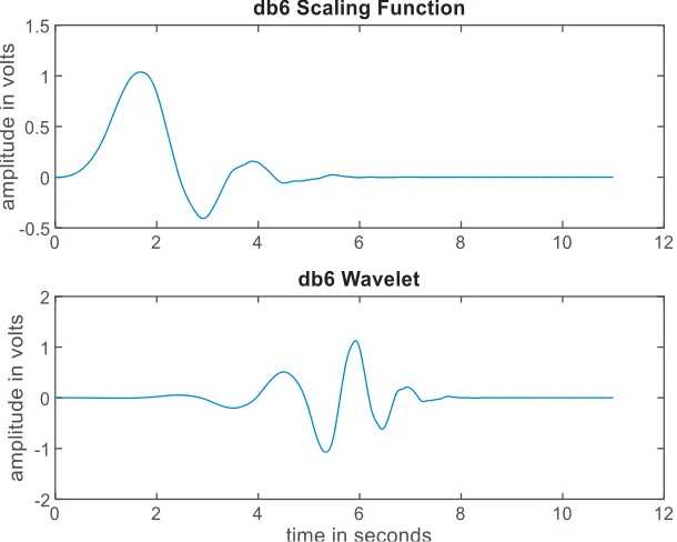
Three-dimensional wavelet functions are used to present the basis functions. These functions estimate the solutions of integral equations. Daubchies 6 wavelet is an orthogonal wavelet with compact support and is used in different numerical approximation problems.

Received 21 April 2018, Accepted 9 June 2018, Scheduled 28 June 2018

* Corresponding author: Manisha Khulbe ([email protected]).

1 _{Department of Electronics and Communication Engineering, Amity School of Engineering and Technology, Amity University,}

The nonlinearity and susceptibility of a medium play an important role in the generation of second harmonic and third harmonic waves, which is used in imaging [4–6]. Terahertz technology is also applied to image processing using a minimum entropy criterion for estimating and compensating linear phase error [2]. By the nonlinear interaction of light and matter, THz waves are produced. These THz waves can be used in nondestructive detection, medical imaging and standoff personnel screening [2]. A two-dimensional imaging of CW THz radiation using electro-optical detection was done by Nahata et al. [4]. A 3D imaging system was worked out by Chattopadhyay et al. [6] involving THz sources and heterodyne detection techniques in submillimeter frequency modulated carrier wave.

In this work, we consider a slab of inhomogeneous medium. An algorithm is given to find the medium parameters susceptibility and permeability in terms of scattered electromagnetic fields. Using wavelet basis functions in least square estimation and inner product method using Method of Moment, the inverse solutions and parameters are obtained in terms of basis functions.

Paper organization is as follows. In Section 2, computational algorithms is given to estimate the parameters of a medium in terms of time domain algorithms using first order susceptibility. Section 3 defines the algorithm using second order susceptibility, and Section 4 gives the wavelet solutions for integral equations. In Section 5 the parameter estimation method Least square estimation and Inner product methods are defined. Stochastic method is also derived for random parameter estimation. Section 6 shows result and simulation where the results of least square estimation and inner product are shown. Section 7 concludes this work.

2. COMPUTATIONAL ALGORITHMS TO ESTIMATE THE PARAMETERS OF A MEDIUM

2.1. Time Domain Algorithm for First Order Susceptibility

In majority of inverse scattering algorithms, the illumination of an object or medium is done by an incident wave which may be generated by an array of antennas or an ultra-wideband pulse [8]. For analyzing we need a setup to use time domain solver [1]. Using the computer model forward scattering data are generated.

Forward Solver:

An electromagnetic wave is incident on the medium. Maxwell’s equations are written for the medium, which gives nonlinear Helmholtz equation [9] in terms of electric E and magnetic field H. Here susceptibility kernel of the medium is assumed on some prior approximate data for the forward solver in computer model. Generalized Helmholtz equation is obtained for electric as well as magnetic fields of a nonlinear random medium. In the forward solver of computer program we can approximate the scattered waves E1, H1, E2,H2 in terms of the incident electric or magnetic fields. For this, we need some basic knowledge of the scatterers. For this calculation a set of Maxwell’s equations are derived changing the permeability and permittivity of the medium to inhomogeneous parameters of the medium.

This method includes two parts:

1. Using integral equation formulation of linear PDE or solving PDE.

2. Equations are resolved in terms of Green’s function and method of moment. From Maxwell’s equations —

∇(E) = 0 (1)

Here we assume that permittivity χe(x, y) and permeability χmn(x, y) both are functions of x, y and

are perturbed by δ then

μ(x, y) = μ0(1 +δχmn(x, y)) (2)

(x, y) = 0(1 +δχe(x, y)) (3)

δ is a small amount of perturbation due to applied electric field.

E = E0+δE1+δ2E2+. . . [1] (4a)

In Equation (1), we put Equations (3) and (4) —

div(0(1 +δχe))

E0+δE1+δ2E2+. . .= 0 (5)

From Equation (5), we get

0divE0 = 0 (6)

divE1+∇χe,E0

= 0 (7)

χe = χe(x, y)

0

divE2+∇χe,E1

+χedivE1 = 0 (8)

Opening Maxwell’s equation for magnetic field —

∇ ·(B) = 0 (9)

∇ ·(μH) = 0 (10)

μ = μ0(1 +δχm(x, y)) (11)

∇ ·(μ0(1 +δχm(x, y))H) = 0 (12)

If the field H is perturbed by δ then again use Taylor series expansion in H. We putH= (H0+δH1+δ2H2+. . .)) in Equation (12)

∇ ·(μ0H) =∇

μ0

1 +δχmn(x, y)

H0+δH1+δ2H2+. . . = 0 (13) δ∇ ·μ0H0

= 0 (14)

δ1μ0

Div·H1+∇χmn(x, y)H0

= 0 (15)

∇ ·μ0H2+∇

χmn·H1

= 0 (16)

Div·H2+∇χmnH1

+χmn∇H1 = 0 (17)

Using curl equations —

∇×(∇ ×E) =∇ ×(−jωμH) =−J (18)

∇(divE)− ∇2E=−jω( (∇μ)×H+μ∇ ×H) (19) ∇2

E− ∇(divE) +jω(∇μ0(1 +δχm)

×H0+δH1+δ2H2+μ0(1 +δχm)∇ ×(H0+δH1+δ2H2+. . .)) = 0 (20)

The following equation is written in the form of permittivity and permeability functions, which will vary as a function ofx,y. We should have prior knowledge of the scatterers so as to generate computer based data or forward solution.

Substituting

∇ ×H=jωE (21)

we get —

∇2_{E− ∇(divE) +jω∇μ}

0(1 +δ∇χm)×(H0+δH1+δ2H2+. . .)

−jωμ(jω0(1 +δχe(x, y)) (E0+δE1+δ2E2 +. . . .) = 0 (22)

Solving Equation (19) we getE1_,E2_,H1_,H2 _{in terms ofE}0 _andH0

∇2

E0+K2E0 = 0 (23)

∇2

E1+∇∇χe, E0

−jωμ0∇χm×H0+K2

χmE0+χeE0

+K2E1 = 0 (24)

In medium, we get perturbation in electric field in terms of the fundamental field E0 [10].

If initial electric field is taken as radiation from a small dipole, Green’s function and current density are assumed equal to 1 [10]. Then

E0(t, r) =

f

ˆ

n, t−n, rˆ c

dΩ (ˆn) which is equal to

The perturbed electromagnetic field is given by Taylor series expansion — (Using duality E→H,H→ −E,→μ)

Forδ0

∇2_H0_+K2_H0_{= 0 (26)}

Forδ1 ∇2

H1+∇∇χm, H0

−jωμ0∇χe×E0+K2H1+K

2

(χm+χe)E0 = 0 (27)

∇×(∇×H) =∇×(−jωE) =−jω(∇×E+∇×E) =−jω(∇×(1+δχe)×E)+(1+δχe) (∇×E) (28)

∇2_{H− ∇(∇ ·H) =−j∇×}

0(1+δχe)

E0+δE1+δ2E2+. . .+0(1+δχe)(−jωμH)}

= jω∇×E0+δ∇×χe

E0+δE1+δ2E2+. . .+j2ω2μ00(1+δχe)(1+δχm)

H0+δH1+δ2H2+. . . (29) ∇2_(H0_+δH1_+δ2_H2_{+. . .)− ∇∇ ·H}0_+δH1_+δ2_H2_{+. . .=RHS (30)} ∇2_H0_+K2_H0 _{= 0}

∇2

H1+K2H1=∇∇·H1−jω0

∇×χeE0

−K2χmH0+χeH0

(31)

∇H1=−∇ ·(χmH0) put in Equation (31)

∇2

H1+K2H1=−∇∇χm,H0

+K2(χm+χe)}+jωμ0

∇ ×χeE0

(32)

Same equation exists for H1 — Hence using

E0(r) =

E0(k)exp(−jkr)d3r (33)

which is perpendicular to the direction of propagation hence using (k, E0(r)) = 0

∇×E0(r) =−jωμH0 (34)

From above equation incident magnetic field isH0 which is computed —

H0 =

P

1

Kα×E0(Kα)

ωμ0

(35)

E1 using Green’s function will be evaluated in terms ofE0, similarly, E2 in terms of E0 and iterative solution in terms of lower order fields.

E1=−

Gk

r−r∇∇χe,E0

r+jωμ0

∇χm×H0

r+K2χe

r+χm(r)

E0rd3r (36)

ThisE1 is in terms of E0 and H0. Similarly, for E2

∇2

E2− ∇divE2+jω∇×χmH1

−j2ω2μ00

χe

rχm

rE0r +K2E2+K2(χe

r+χm

rE1) = 0 (37)

From Equation (7) —

0divE2 =−0∇(χeE1)−0χedivE1 (38)

Put in Equation (38)

∇2

E2+∇∇χe

r,E1r+χe

rE1r+K2E2 = −jω∇ ×χm,H1

−K2(χm+χe)E1−K2χeχmE0 (39)

So

∇2₊

K2E2=−∇∇χe,E1

+χe

∇·E1−jω∇×χm,H1

−K2(χm+χe)E1−K2χeχmE0 (40)

Ifχm = 0 for nonmagnetic material, then equation is reduced to

∇2₊

K2E2=−∇∇χe,E1

+χe

∇·E1−K2(χm+χe)E1 (41)

E2=−

Gk

r−r∇∇χe,E1

r−jωμ0

∇χm×H1

r+K2χe

rE1rd3r (42)

E2 is in terms ofE1 and H1.

In Equation (24), also if χm = 0, the material is assumed as nonmagnetic, and the equation is

reduced to

∇2

E1+K2E1

=−∇∇χe, E0

(r) +K2χeE0

(43)

First order-perturbed field in terms of the Green’s function is written as —

E1 = −

Gk

r−r ∇∇χe, E0 ω, r

+K2χeE0 ω, r

d3r (44)

E1(ω, r) = − 1 4π

e−jk(r−r) |r−r|

∇∇χe, E0 ω, r

+K2χeE0 ω, r

d3r (45)

Hence E1 and E2 are iterative solutions where E1 depends on E0, and E2 depends onE1. So if E1 is calculated, we can put the values in Equation (43) to calculate E2. However for a magnetic material, the computations are a bit lengthy.

Similarly, H2 can be calculated from Equations (29), (30) and (31). In terms ofχm, χe

∇2

H2+K2H2 = ∇∇ ·H2−jω0

∇ ×(χeE1

+j2ω2μ00(χm+χe)H1+j2ω2μ00(χmχe)H0 (46)

∇2_H2_+K2_H2 _{= −μ} 0

∇χmH1

+χm∇·H1

−jω0

∇×(χe, E1

−K2χeχmH0−K2(χe+χm)H1(47)

=μ0∇∇·χm,H1

+χm∇·H1

+K2(χe+χm)H1+jω0

∇×χe, E1

+K2χeχmH0

(48)

Equations (46) and (33) tell us how to compute the first order scattered fields E1_{, H}1 _{from the} incident fieldsE0,H0, and Equations (43) and (47) tell us how to compute the second order scattered fields E2, H2 that is the next higher order corrections to the scattered fields in terms of E0, H0 and E1,H1. We have been using second order perturbation theory.

3. FORWARD SOLVERS IF THERE IS A SECOND ORDER SUSCEPTIBILITY χ2

divE+δχ1E1+δ2χ2E2±. . .= 0 [11]

Using Einstein summation convention over spaceβ is defined as

χ2(E⊗E)(ω, r) =

χ2(ω1, ω−ω1, r)(E(ω1, r)⊗E(ω−ω1, r))d ω1 (49)

=

χ2_αβγ(ω1, ω−ω1, r)E_β(ω1, r)Eγ(ω−ω1, r)d ω1

α

(50)

α, β, γ are the indices.

Again Einstein summation convention over (βγ) is implied

E =E0+δE1+δ2E2+O(δ3) (51)

divE0= 0,

divE1+ divχ1·E0= 0, (52)

divE2+ div(χ1E1) + div(χ2E0⊗E0) = 0 (53)

χ1_αβ(ω, r) =

N

m=1

θ_αβm1 ψ1_m(ω, r) (54)

χ2_αβγ(ω1, ω2, r) =

N

m=1

Remark1:The coefficientsθ1_αβmandθ2_αβγmin these expressions are the parameters to be estimated. ψ_km1 , ψ_km2 known as basis functions.

IfE0 is represented by —

E0(ω, r) =

F(ω,nˆ) exp (jkˆn·r)dΩ (ˆn) (ˆn, F(ω,nˆ)) = 0 (56)

(Since divE0 = 0)

∇ ×E = −jωμH (57)

∇ ×H = jω0(E+δχ1E+δ2χ2(E⊗E)) (58)

∇ ·H = 0 (59)

Hence

∇(∇ ·E)−∇2E=k2(E+δχ1E+δ2χ2(E⊗E)) (60)

Propagation constant k2=ω20μ (61)

∇2_E0_+K2_E0_{= 0, (62)}

∇2

E1+K2E1+k2χ1E0+∇divχ1E0= 0, (63)

∇2

E2+k2E2+k2χ1E1+k2χ2E0⊗E0+∇divχ1E1+∇divχ2E0⊗E0= 0 (64) Equations are represented in the form of basis function and parameter variation defined in indices.

In Equation (37), we put susceptibility in matrix form and define it in terms of indicesαβγm

E_α1(ω, r) =− 1 4π

Gω

r, rχ1_γβω, r, E_β0ω, r, γαd3r+K2χ1_αβω, rE_β0ω, rd3r (65)

Remark2: 1 — A symbol like F(ω, r),_η means ∂F_∂X(ω,rη ) η= 1,2,3.

and a symbol like _∂X∂2Fη(_∂Xω,rα) means η, α= 1,2,3.

2 — All through here calculates the indices αβγk run over 1, 2, 3 and we adopt the summation convention, i.e., if a repeated index appears then it means we are summing over that index.

Defining a susceptibility matrix in the form of wavelet basisψ1_{(ω, r) function, we can express the} scattered signal as —

E_α1(ω, r) = −

k,γ,β

θ_γβk1 ψ_k1(ω, r), E_β0ω, r, γαd3r

+δγαK2ψk1

ω, rE_β0ω, rGω

r, rd3r (66)

θ1_γβk are parameters in terms of wavelet coefficients. Green function

Gω

r, r= e

−ik|r−r|

4π|r−r| (67)

Or if electromagnetic field in frequency domain is given by

E_α1(ω, r) =

αβγ

θ1_γβk

Fβ(ωnˆ)dΩ(ˆn)

× δγαk2ψk1

ω, reiknˆ·r+

ψ1_kω, reiknˆ·r

,

αγ

Gω

r, rd3r (68)

E_α1(ω, r) =

αβγ

θ1_γβk

Fβ(ωnˆ)dΩ(ˆn)

× k2δγαψ1k

ω, reiknˆ·r +ψ1_k,γω, reiknαˆ −ψ1_k,γω, rk2nαnγ

eikˆn·r

Gω

We can write this as —

E_α1(ω, r) =

αβγ

θ1_γβk

Fβ(ω,nˆ)Kαγ

ω,nˆαr

(70)

where

Kαγ

ω,nˆα,r

=

k2ψ1_k,γω,r(δγα−nαnγ) exp

jknˆ·rGr,rd3r

+

jkψ_k,α1 ω, rny+ψ1k,γ

ω, rnα

exp(jknˆ·r))Gω

r,rd3r

+

ψ_k,αγ1 ω,rexpjknrˆ Gω

r,rd3r (71)

nis a unit vector representing direction defined for a region L.

The above equations give the forward solver data and it as an iterative process. Other higher order fields can also be calculated.

4. WAVELETS FOR NUMERICAL SOLUTIONS OF INTEGRAL EQUATIONS

The integral equations provide an important tool for modeling a numerous phenomenon and processes. Many numerical methods have been developed for one-dimensional integral equation, and fewer methods are known for two- and three-dimensional integral equations.

Many different basic functions are used to estimate the solution of integral equations, such as orthogonal functions and wavelets. Daubchies wavelets are orthogonal wavelets with compact support, and they have been used in different numerical approximation methods [14].

The orthogonal basis ψn(t) of one-dimensional Daubchies wavelet for the compact support space

L2[0,10] consists of

ψk,n(t) =|a|−

1 2 _ψ

ak0t−nb0

[0,1] (72)

wheren= 1,2. . . ,0≤k≤2n−1.

It forms a basis forL2(R)·a0 = 2 and b= 1.

In this work we apply three-dimensional Haar wavelet construction on [0,10]×[0,10]×[0,10] to solve the least square estimation method and inner product method.

The integer 2k indicates the level of the wavelet, and nk0 is the translation parameter. By simple

calculations

1

0

ψm(r)ψn(r) =

1 m=n

0 m=n (73)

Any functionψn(x)∈C[0,1] can be expressed [12] as

n f, ψn ψn

where

f, ψn =

1

0

f(r)ψn(r)dr (74)

If ψk(r) is a basis function which is one-dimensional wavelet on [0,1], then for three-dimensional

analysis we have taken the same wavelet in three dimensionsx,y,z.

The expansion off(x, y, z) is defined over [0,1]×[0,1]×[0,1] expanded by the three dimensional Daubchies wavelet Db6.

For simplification we assume that if wavelet basis is as ψk(r), then define susceptibility and

permeability in one dimension as —

χe

r=

d

1

akψk(r) And χm

r=

d

1

bkψk(r) (75)

ak, bks are constants. For three dimensions we take summation in the given region space integrating

Substitutingχe(r) by above values in Equation (37), the fields are solved in terms ofE0 and H0. For simplification letak andbk be assumed parameters of the medium (as measured values will be

depending on it). Both E1_{(r) and H}1_{(r) are written in the form of E}0 _{and H}0 _{from Equations (33)} and (46).

E1(r) =

d

k=1

akλ1k(r) + d

k=1

bkλ2k(r) (76)

E1(r) is the scattered field, and λ1_k(r), λ2_k(r) are the integral equations in terms of E0 and H0, respectively. Similarly, forH field

H1(r) =

d

k=1

akλ3k(r) + d

k=1

bkλ4k(r) (77)

H1(r) is the scattered field, and λ3_k(r), λ4_k(r) are the integral equations in terms of E0 and H0, respectively.

We have E0 and H0 expressed in terms of wavelets.

H0 =

p

1

αkE0(kα)

ωμ0

(78)

λ1_k(r) = −

Gk

r−r ∇∇χe, E0 r

+K2χe+χm

rE0(r)d3r (79)

λ2_k(r) =

Gk

r−r jωμ0

∇χm×H0 r

d3r (80)

λ3_k(r) =

Gk

r−r jωμ0

∇×χe,E0

d3r (81)

λ4_k(r) = ∇∇χm,H0

+K2(χm)H0

d3r (82)

In the first experiment, we assumeχe&χm a matrix and calculate the scattered outputs. In our earlier

work, this has been taken as centrosymmetric and noncentrosymmeric matrices, and the scattered outputs were calculated [13].

First order scattered fieldsE1 andH1 and second order scattered fieldsE2 and H2 are calculated (Figure 1 [13]) using Maple.

5. PARAMETER ESTIMATION METHODS

5.1. Least Square Estimation

The scattered or measured data are as follows — which depend upon two parameters — θ1, θ2 of the medium [14]

E0(t, r) = θ1X1

r+θ2X2

r, (83)

E1(t, r) = θ1F1(ˆr) +θ2F2(ˆr) (84)

In order to find the error between the measured data and computer generated data, by applying least mean square error [14]

kE

1₍

ω,rˆk)−α1F1(ˆrk)−α2F2(ˆrk)

2

=Xn (85)

The minimization of the equation uses Eq. (86) —

akbk

⎧ ⎨ ⎩w1j

E1(rj)− d

k=1

akλ1k(rj)−bkλ2k(rj)

2

+w2j

H1(rj)− d

k=1

akλ1k(rj)−bkλ2k(r)

2⎫_⎬

Figure 1. Db6 wavelet (using Mat lab).

Minimization and approximation are done by taking the derivative of error with respect to parameters X1 and X2, and we get the matrix and set it to zero.

Then

k

_E1_{(t, r)−α}

1F1(ˆrk)−α2F2(ˆrk)

2

=Yn (87)

Finding dYn dα1

and dYn dα2

and setting it to zero (88)

Parameters are defined in terms ofα1 and α2.

We getα1α2in terms ofF1(ˆr) andF2(ˆr) in matrix form. These are the parameters of the nonlinear material

α1 α2

_T

= argmin_(α1α2)

l≤k≤p

(WψY)nk,l

−(WψY)T_nk,l

2

= ⎡ ⎣

n,k

(WψX)_nk,l(WψX)T_nk,l

⎤ ⎦

−1⎡ ⎣

k,l

(W_ψY)

nk,l

⎤

⎦ (89)

Error minimization leads to the following matrix

− ⎡

⎣ 2X1(ˆrk)

2 ₂

kRe (X1(ˆrk)X2(ˆrk))

2

kRe(X1(ˆrk)X2(ˆrk)) 2X2(ˆrk)

2

⎤ ⎦

−1 ×

⎡

⎣ 2 kRe

E1(ˆrk)X1(ˆrk)

2

kRe

E1(ˆrk)X2(ˆrk)

⎤ ⎦

(90) The fields are in terms of magnetic component and electric field components. Error minimization is done by the following equation —

Minimizing

akβkw1j

E1(rj)− d

k=1

akλ1k(rj)− d

k=1

bkλ2k(rj)

2

+w2j

H1(rj)− d

k=1

akλ3k(rj)− d

k=1

bkλ4k(rj)

2

(91)

5.2. Inner Product with Integral Equations

Another method is by taking inner product of fields generated by forward solver of E1, H1 to λ1_m(rj)

andλ3_m(rj), respectively. It is also used as a basis function as scattered waves are presented in its form.

Here we get two sets of equations for E field and H field.

E1(rj), λ1m(rj)

! =

d

k=1

ak λ1k(rj), λ1m(rj)

! +

d

k=1

bk λ2k(rj), λ1m(rj)

!

(92)

H1(rj), λ3m(rj)

! =

d

k=1

ak λ2k(rj), λ3m(rj)

! +

d

K=1

λk λ4k(rj), λ3m(rj)

!

(93)

By adding them, we get the following equations —

RHS of the following equation generates data in a forward solver called computer-generated data where fields are represented in the form of integral equations. It is an inner product between integral equations.

From Equations (93) and (94) —

K

j=1

w1j E1(rj), λ1m(rj)

! +

K

j=1

w2j H1(rj), λ3m(rj)

! = d K=1 ak K j=1

w1j ηk1(rj), ηm1 (rj)

! + d K=1 ak K j=1

w2j ηk2(rj), η3m(rj)

! + d K=1 bk K j=1

w1j ηk2(rj), η1m(rj)

! + d K=1 bk K j=1

w2j η4k(rj), ηm3 (rj)

!

(94)

This gives a scattered field matrix

ξE = AEEα+AEHβ (95)

ξH = AHEα+AHHβ (96)

In addition, parameters can be calculated by using inverse ofAmatrix with the scattered field matrix. α β =

AEE AEH

AHE AHH

ξE

ξH

(97)

where field matrix scattered is multiplied with the integral equations λ1_m(rj) in time domain.

αk

βk

λ1_k(rj),λ1m(rj)

!

λ2_k(rj), λ1m(rj)

!

λ2_k(rj), λ3m(rj)

!

λ4_k(rj), λ3m(rj)

! = ξE ξH (98) αk βk =A−1

ξE ξH

(99)

ξE =

K

j=1

w1jE1(rj), λ1m(rj) (100)

ξH =

K

j=1

w2jH1(rj), λ1m(rj) (101)

Here again putχm= 0 for a nonmagnetic material.

E1η1_k!+ H1η_k3!= [ ak bk ]

"

wi akλ1_k(r), akλ1_k(r)

!

wij = 0

w2j akλ1_k(r), akλ1_k(r)

!

w2j akλ3_k(r), akλ4_k(r)

! #

We get — _akλ1

k(r)

2

=∇∇χe, E0 r

+K2(χe)E0(r)

2

(103)

akλ1k(rj), akλ2k(rj)

!

= 0 (104)

_akλ3

k(rj)

2

=|jω0∇ ×χe, E|2 (105)

a2_kλ3_k(rj), λ4k(rj)

!

= (iω0∇ ×χe, E)

∇∇χm,H0

+K2(χm+χe)H0

whereχm= 0 (106)

[ AEE AEH

AHE AHH ] is a computer generated forward solver. [

ξE

ξH ] is the measured scattered field inner

product with the basis functions. [ α

β ] are the parameters of the medium. Future Scope

5.3. The Statistical Parameters of the Random Medium Over Dimension L

Nonlinear medium behaves as a harmonic oscillator [5], and the scattering is random. Random variables whose matrix is estimated are calculated by estimating the mean value ofE(ω, r) and correlations using local ergodicity. Ensemble averages can be replaced by local frequency and spatial averaging defined by correlations of the scattered fields. If θγβm are random variables whose statistics is to be estimated,

then we find the expectationE(θγβm) andE(θγβmθγβm) estimating the mean value ofEα(ωr) and its

correlations using local ergodicity. Here ensemble averages are replaced by local frequency and spatial averages.

E[E_α(ω, r)] = Eθ_γβmLαβγm(ω, r) (107)

And

EE_α (ω, r)E_αω, r=

αβγmαβγm

Eθ_αγβmθ_αγβmL_αγβm(ω, r)L_{αγβmω, r} (108)

whereE_α(ω, r) =

γβm

θγβmLαβγm(ω, r).

From Equation (69)

Lαβγn(ω, r) =

Fβ(ω,nˆ) αβγ

θ_γβk1

Fβ(ω,ˆn)dΩ(ˆn)

× δγαk2ψk1

ω, reiknˆ·r+

ψ1_kω, reiknˆ·r

,

αγ

Gω

r, rd3r (109)

The aim here would be to evaluate the mean and covariance of parameters θ1_βkγ from the mean and covariance of the scattered electric fields. The mean and covariance of the electric field can be estimated using spatial and frequency averages assuming ergodicity.

Here we assume that the parameters are θ. For example

EE_α(ω, r)E_αω, r≈ 1 N

ξ,η∈B

E_α (ω+ξ, r+η)E_αω+ξ, r+ηdξdη , (110)

whereN =$_Bdξdη.

This is the expansion of the scattered electric field in terms of susceptibility expansion coefficients θγβm, which are assumed to be random variables for characterizing the randomness of the susceptibility

6. RESULTS AND SIMULATIONS

6.1. Inner Product with Integral Equations Defined by

E1, λ1_m! (111)

Using wavelet basis functions — ψk is a basis function.

Find ∇ψk first, then take inner product with E0

E0 = ψk (112)

Ifr is a vector space r= ˆx+ ˆy+ ˆz

∇ψk(r) = ∂

∂xψx+ ∂ ∂yψy+

∂

∂zψz (113)

(∇(∇ψk(r)) = ∂

∂x2 2

ψk+ ∂

∂x ∂ ∂yψk+

∂ ∂x

∂ ∂zψk+

∂ ∂y

∂ ∂xψk

+ ∂ ∂y2

2

ψk+_∂y∂ _∂z∂ ψk+_∂x∂z∂

2

ψk+_∂y∂ _∂z∂ ψk+ ∂

∂z2 2

ψk (114)

From Equation (100) are computer generated data from forward solver, and [ ξE

ξH ] are measured scattered field.

In step one we define susceptibility χe and permeability χm of the medium in terms of wavelet

basis functions.

χe(r) = d

k=1

akψk(r) (115)

In direct least square-based estimation on spatial samples at points,r1, r2, r3, . . . , rN we get parameters

by using the equation

ˆ θ1,θˆ2

_T

= argmin_(θ1,θ2)

N

k=1

Y (rk)−θTX(rk)

2

= % _N

k=1

(X(rk)X(rk)T

&−1% _N

K=1

Y (rk)X(rk)

&

(116)

Heavy computations are required for large N. On the other hand, if we know that parameters X1(r), X2(r) have dominant wavelet coefficients at the resolution indices {n1, n2, np} only then, we

can use the model.

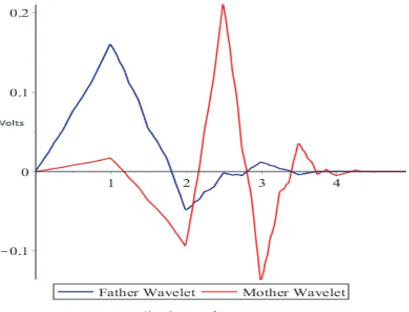
Basis function Daubchies wavelet (see Figure 1) is designed in Matlab and in Maple (see Figure 2). Initially the scattered electromagnetic fields are E1, E2 simulated in Maple [13].

6.2. Outputs Using Least Square Estimation

Using least square estimation method, we estimated state space representation of the susceptibility and permeability [14].

The incident electric and magnetic fields were designed, and scattered electric fields are simulated using self-phase modulation, which is defined by third order nonlinearity [14].

Figure 2. Wavelet basis function Db6 using Maple tool.

and above-mentioned methods can be used in imaging 1D, 2D and 3D data. Figures 1 and 2 give the Daubchies wavelet and its matrices in the workspace.

psi(s) = W avelet Coef f icients(“Daubechies”, 6)

Ψ(x) = ⎛ ⎜ ⎜ ⎜ ⎜ ⎜ ⎝ ⎡ ⎢ ⎢ ⎢ ⎢ ⎢ ⎣

0.0352262918857095 0.0854412738820267 −0.135011020010255 −0.459877502118492 0.806891509311093 −0.332670552950083

⎤ ⎥ ⎥ ⎥ ⎥ ⎥ ⎦·

⎡ ⎢ ⎢ ⎢ ⎢ ⎢ ⎣

0.332670552950083 0.806891509311093 0.459877502118492 −0.135011020010255 −0.0854412738820267

0.0352262918857095 ⎤ ⎥ ⎥ ⎥ ⎥ ⎥ ⎦

⎞ ⎟ ⎟ ⎟ ⎟ ⎟ ⎠

The scattered fields are calculated at 4.7 GHz [14] frequency. Figure 3 gives the scattered field amplitude and phase variation, which is fed to Equation (90).

The least square estimation gives permeability and permittivity variations shown in Figures 4(a) and 4(b).

6.3. Outputs Using Inner Product Methods

A set of equations from (96) to (101) are used to find the inner product solutions. Scattered electromagnetic wave from self-phase modulated data [13] is used which is a nonlinear scattered electromagnetic wave. UsingEandHfields from these second order nonlinear waves and defining three-dimensional wavelet basis functions for susceptibility, we get the set of equations. Equations from (103) to (107) are used for inverse solutions. Assuming negligible magnetic permeability, susceptibility variations are calculated. Figure 5 shows the relative susceptibility variation in the medium.

6.4. Discussions

(a)

(b)

Figure 3. Scattered waves E1 _{generated by self-phase modulation for testing the inverse technique} (Figure 3 [14]). (a) Impulse response. (b) Magnitude and phase response.

as well as limited number of frequencies is done. It has been studied that the solution is not unique for practical problems, and uniqueness of the integrating field is overcome by measuring large number of samples of the scattered field data [7]. We estimated susceptibility by the least square estimation method. The error between the measured values and computer-generated values is practically used to optimize parameters of the medium. This RF imaging technique is helpful in identifying the hidden objects and underground explosives, which can be used for security purposes.

(a) (b)

Figure 4. Spatial resolution of medium parameters at 4.7 GHz (Figure 4 [14]). (a) Relative susceptibility variation. (b) Relative permeability variation.

Figure 5. Relative susceptibility variation assuming medium is nonmagnetic using inner product method.

by treating the susceptibility tensor as being the first order of smallness, we express the first order perturbation to the electric field (i.e., the scattered field) as a linear combination of these expansion parameters. To do so, Green’s function for the Helmholtz operator is used.

7. CONCLUSION

Using Maxwell’s equations, we have optimized the parameters of an inhomogeneous medium by scattered electromagnetic fields with a time domain algorithm. The inverse solutions using Least Square Estimation and Inner Product Methods are solved by method of moments. Parameters are obtained in terms of the basis functions. Forward solver technique is used with the first order nonlinearity and Kerr nonlinearity. Method of moment is used with wavelet bases in one-dimensional, two-dimensional and three-dimensional cases. For this, we use two-dimensional and three-dimensional wavelet functions. Computational complexity increases as the number of wavelets is increased. We can limit this problem by taking a limited number of wavelets for a set of scattered electromagnetic waves, which will reduce the computational cost. Wavelet technique requires less memory space. Wavelet basis also gives better solutions in terms of fast computations. To conclude, we have developed a computationally cheaper algorithm for estimating linear and nonlinear components of the parameters that govern the susceptibility field from measurements of the scattered Electromagnetic fields at different frequencies and spatial locations.

REFERENCES

1. Seema, N., A. Sabouni, T. Desell, and A. Ashtari, Microwave Tomography, Global Optimization Parallelization and Performance, Springer, 2014.

2. Gao, J. K., Y. L. Qin, B. Deng, H. Q. Wang, J. Li, and X. Li, “Terahertz wide angle imaging and analysis on plane wave criteria based on inverse synthetic aperture techniques,” J. Infrared Milli. Terahertz Waves, Vol. 31, 373–393, 2016.

3. Shea, J. D., B. D. Van Veen, and S. C. Hagness, “A TSVD analysis of microwave inverse scattering for breast imaging,” IEEE Transactions on Biomedical Engineering, Vol. 59, No. 4, 936–945, Apr. 2012.

4. Nahata, A., J. T. Yardley, and T. F. Heinz, “A two dimensional imaging of CW THz radiation using electro-optic detection,” Applied Physics Letters, Vol. 81, No. 6, 963–965, Aug. 2002.

5. Khulbe, M., H. Parthasarathy, and M. R. Tripathy, “Mathematical analysis and design of RF imaging techniques and signal processing using wavelets,” International Journal of Signal and Imaging System Engineering, Inderscience Journal, Vol. 10, No. 6, 2017.

6. Chattopadhyay, G., C. Dengler, T. E. Bryllert, E. Schlecht, A. Skalare, I. Mehdi, and P. H. Siegel, “A 600 GHz imaging radar for contraband detection,” 19th International Symposium on Space Terahertz Technology, 300–303, Groningen, Apr. 28–30, 2008.

7. Brasselel, S., “Polarization resolved nonlinear microscopy Applications to structure molecular and biological imaging,”Advances in Optics and Photonics, Vol. 3, 205–271, 2011.

8. Kumar, A., A. Basu, and S. K. Kaul, “Circuits and active antennas for ultrawide band pulse generation and transmission,”Progress In Electromagnetic Research B, Vol. 23, 251–272, 2010. 9. William, W. H., W. C. Chew, and C. A. Ruwe, “A step frequency radar system for broadband

microwave inverse scattering and imaging,” Review of Progress in Quantitative Nondestructive Evaluation, 643–649, Springer, 1995.

10. Balanis, C. A.,Antenna Theory Analysis and Design, 2nd Edition, Wiley, 1997. 11. Robert, B. W., Nonlinear Optics, 3rd Edition, Elsevier, 2008.

12. Derili, H. A., S. Schrabi, and A. Arzhang, “Two dimensional wavelets for numerical solution of integral equations,” Mathematical Sciences, 2, 5, 6, 2012.

13. Khulbe, M., H. Parthasarathy, and M. R. Tripathy, “THz generation using nonlinear optics: Mathematical analysis and design of THz antennas,” Advanced Electromagnetics Journal, Vol. 7, No. 1, Feb. 2018.