Quantitative Analysis of Three-Dimensional Cone-Beam Computed Tomography Using Image Quality Phantoms

(1)

Scholarship@Western

Electronic Thesis and Dissertation Repository

10-25-2018 2:00 PM

Quantitative Analysis of Three-Dimensional Cone-Beam

Computed Tomography Using Image Quality Phantoms

Rudy Baronette

The University of Western Ontario Supervisor

Holdsworth, David W.

The University of Western Ontario Co-Supervisor Teeter, Matthew G.

The University of Western Ontario

Graduate Program in Medical Biophysics

A thesis submitted in partial fulfillment of the requirements for the degree in Master of Science © Rudy Baronette 2018

Follow this and additional works at: https://ir.lib.uwo.ca/etd

Part of the Medical Biophysics Commons

Recommended Citation Recommended Citation

Baronette, Rudy, "Quantitative Analysis of Three-Dimensional Cone-Beam Computed Tomography Using Image Quality Phantoms" (2018). Electronic Thesis and Dissertation Repository. 5797.

https://ir.lib.uwo.ca/etd/5797

This Dissertation/Thesis is brought to you for free and open access by Scholarship@Western. It has been accepted for inclusion in Electronic Thesis and Dissertation Repository by an authorized administrator of

(2)

i

Abstract

In the clinical setting, weight-bearing static 2D radiographic imaging and supine 3D

radiographic imaging modalities are used to evaluate radiographic changes such as, joint

space narrowing, subchondral sclerosis, and osteophyte formation. These respective imaging

modalities cannot distinguish between tissues with similar densities (2D imaging), and do not

accurately represent functional joint loading (supine 3D imaging). Recent advances in

cone-beam CT (CBCT) have allowed for scanner designs that can obtain weight-bearing 3D

volumetric scans. The purpose of this thesis was to analyze, design, and implement advanced

imaging techniques to quantify image quality parameters of reconstructed image volumes

generated by a commercially-available CBCT scanner, and a novel ceiling-mounted CBCT

scanner. In addition, imperfections during rotation of the novel ceiling-mounted CBCT

scanner were characterized using a 3D printed calibration object with a modification to the

single marker bead method, and prospective geometric calibration matrices.

Keywords

(3)

ii

Co-Authorship Statement

The following thesis contains manuscripts intended for publication within scientific journals.

Chapter 2 is an original manuscript entitled, “Quantitative Performance Evaluation of a

Peripheral Cone-Beam Computed Tomography Scanner with Weight-bearing Capabilities.”

The manuscript is co-authored by Rudolphe J. Baronette, Xunhua Yuan, Steven I. Pollmann,

Matthew G. Teeter, and David W. Holdsworth. In my role as a MSc candidate, I participated

in designing the study, performed cone-beam CT scans and reconstruction, performed the

effective dose estimation, analyzed all data, performed the statistical analysis, and wrote the

manuscript text. Xunhua Yuan and Steven I. Pollmann advised on study design,

interpretation of the data, and provided editorial input. Matthew Teeter and David

Holdsworth, as the candidate’s supervisors, designed the study, reviewed the results, gave

editorial assistance and provided mentorship.

Chapter 3 is an or original manuscript entitled, “Three-dimensional cone-beam CT

reconstruction in a natural weight-bearing stance using ceiling-mounted x-ray fluoroscopy.”

The manuscript is co-authored by Rudolphe J. Baronette, Steven I. Pollmann, Matthew G.

Teeter, and David W. Holdsworth. In my role as a MSc candidate, I participated in designing

the study, performed cone-beam CT scans and reconstruction, performed the effective dose

estimation, characterized gantry motion, analyzed all data, performed the statistical analysis,

and wrote the manuscript text. Steven I. Pollmann advised on study design, and interpretation

of the data. Matthew Teeter and David Holdsworth, as the candidate’s supervisors, designed

(4)

iii

Acknowledgments

I would like to begin by thanking my primary supervisor, Dr. David Holdsworth, for this

opportunity and his mentorship throughout my graduate education. He has helped me to

increase my understanding of x-ray imaging system, develop a thorough method for problem

solving, improve my communication of my scientific research, and has provided valuable

insight to each of my projects. I would also like to thank my co-supervisor Dr. Matthew

Teeter, specifically for helping to improve my communication, and providing opportunities

to apply clinical skills in the radiostereometric analysis lab. As a member of my advisory

committee, Dr. Trevor Birmingham has provided invaluable clinical insights for applications

and advantages of my work. The accomplishments within this thesis could not have

happened without the support of individuals within the Holdsworth group at Robarts

Research Institute. Specifically, Steve Pollmann, who created numerous programs for me and

was always willing to provide advice on whatever challenge I was facing, and Jeremy Gill

for his help in developing the orbital acquisition protocol, angular encoder, and geometric

calibration in my 2nd_{project. I would also like to thank Dr. Xunhua Yuan, who helped with}

much of the geometric calibration work, gave me a comprehensive background in

radiostereometric analysis, and was always willing to share his scientific wisdom. Finally, I

would like to thank my family and friends for their support during this journey. This includes

my parents Gary and Kathy, my sister Savannah, my brother Oliver, my aunt Simone, and

(5)

iv

List of Abbreviations

2D two-dimensional

3D three-dimensional

ADU analog-to-digital unit

AINO adaptive imaging noise optimization

BMD bone-mineral density

CBCT Cone-beam computed tomography

CT computed tomography

CTDI computed tomography dose index

FOV field-of-view

GRAIL gait real-time analysis interactive lab

HU Hounsfield unit

kVp kilovoltage peak

LAC linear attenuation coefficient

lp/mm line pairs per millimetre

mA milliamperes

mAs milliampere seconds

MBRSA model-based radiostereometric analysis

mm millimetre

(6)

v

MTF modulation transfer function

NSAIDs non-steroidal anti-inflammatory drugs

OA osteoarthritis

PLA polylactic acid

ROI region of interest

RSA radiostereometric analysis

RSPA roentgen single-plane photogrammetry

TKA total knee arthroplasty

(7)

vi

List of Tables

Table 2.1: Manufacturer’s clinical imaging standards for spatial resolution, linearity,

uniformity, noise, and geometric accuracy. ... 26

Table 2.2: CT numbers (HU) and standard deviation (HU), measured in one central and four

peripheral ROIs for the 300-image projection protocol in the small phantom. Average

difference and average measured standard deviation (±SD) were calculated. ... 38

peripheral ROIs for 450-image projection protocol in the small phantom. Average difference

and average measured standard deviation (±SD) were calculated. ... 38

peripheral ROIs for the 300-image projection protocol in the large phantom. Average

peripheral ROIs for the 450-image projection protocol in the large phantom. Average

Table 2.6: Results of non-linear regression of standard deviations occurring in the small and

large phantoms. The equations are shown in the form, σ2

total = A * E−1 + σ2system, where R2

value for all equations = 0.99. ... 42

Table 3.1: Geometric projection matrices calculated using the calibration algorithm within a

day, summarizing magnitude and reproducibility of geometric imperfections. Geometric

imperfections were reported as the maximum deviation from the average value during

rotation. Geometric reproducibility was defined as the average standard deviation across

multiple acquisitions within a day. ... 73

peripheral ROIs for reconstructed image volumes at the central slice. Average difference and

(11)

x

List of Figures

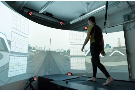
Figure 1.1: Gait real-time interactive analysis lab (GRAIL) located at the Wolf Orthopaedic

Biomechanics Laboratory. ... 3

Figure 1.2: Example of bi-planar setup in the radiostereometric analysis lab located at

Robarts Research Institute. ... 6

Figure 1.3: Radiostereometric analysis calibration cage for a bi-planar examination. ... 7

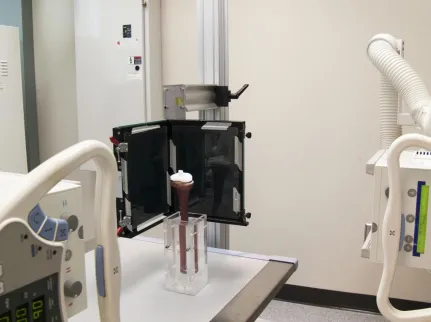
Figure 1.4: NRT Adora X-ray Fluoroscopy system pictured at the Wolf Orthopaedic

Biomechanics Laboratory. ... 9

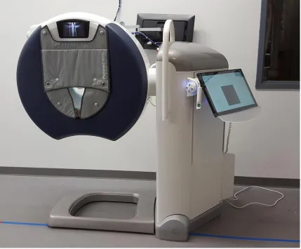
Figure 1.5: Planmed Verity extremity cone-beam computed tomography scanner located at

the Wolf Orthopaedic Biomechanics Laboratory. ... 12

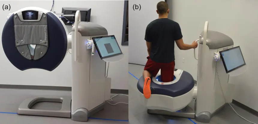
Figure 2.1: Peripheral cone-beam CT scanner pictured in conventional scan (a) mode and

weight-bearing scan (b) mode. ... 24

Figure 2.2: Large custom-built phantom (left) and small phantom (right) designed to evaluate

the performance of cone-beam CT scanners. ... 25

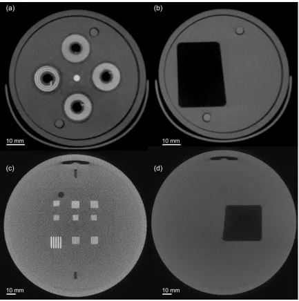
Figure 2.3: Images of small phantom a) resolution coils, created with alternating aluminum

and Mylar sheets, b) the 5° axial slanted-edge image. In the large phantom, c) bar pattern

plate, created with alternating aluminum and Mylar sheets, and d) the axial slanted-edge

image, showing a 5° from the central axis. ... 28

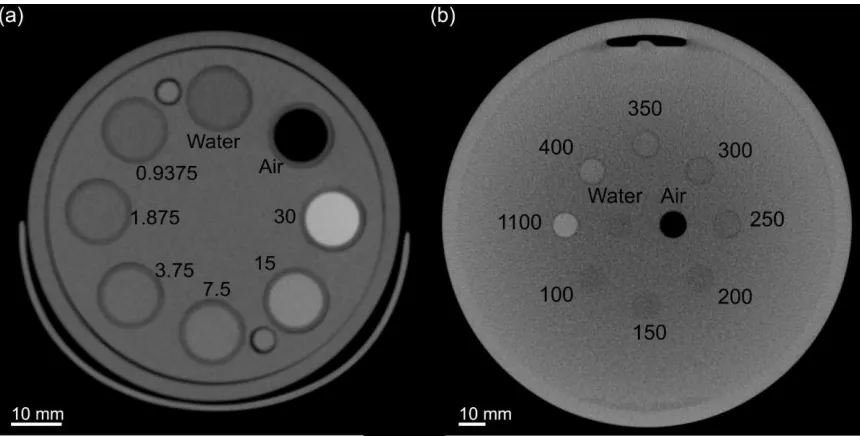
Figure 2.4: Image of linearity plates used in the small phantom (a) containing vials of air,

water, and iodine (Omnipaque) in various concentrations, measured in mg ml-1. Image of

linearity plate in large phantom (b) containing plastics within various bone mineral densities,

measured in mg hydroxyapatite cm-3. ... 29

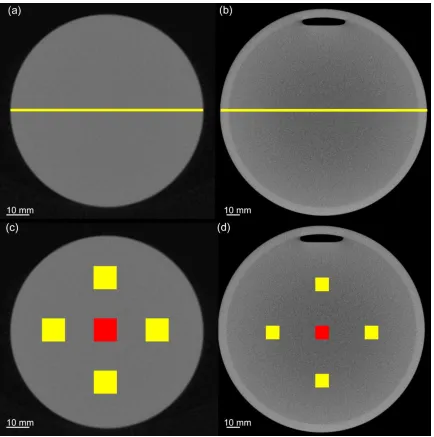
Figure 2.5: Slices through an area of uniform density in the small (a) and large (b) phantoms,

(12)

xi

within the small (c) and large (d) phantoms used to assess uniformity (red & yellow) and

noise (red only). ... 31

Figure 2.6: a) slice from small phantom with five steel beads in axial plane. b) Slices from

large phantom containing: five steel beads in the axial plane, and c) in (x-z) direction with

thirty tungsten-carbide beads spaced 15 mm in all directions. ... 32

Figure 2.7: Modulation transfer function of the cone-beam CT system measured from the

slanted-edge plate (lines) and resolution coils (symbols) of the small phantom using the 6s (a)

and 9s (b) exposure acquisitions. ... 34

Figure 2.8: Modulation transfer function of the cone-beam CT system measured from the

slanted-edge (line) and bar patterns (symbols) in the large phantom, using (a) 6s and (b) 9s

exposures. Additionally, modulation transfer function evaluated with the slanted-edge

located within the x-y plane in the large phantom, using (c) 6 and (d) 9s exposures. ... 35

Figure 2.9: Plots of measured CT number versus known iodine concentrations, including

results of linear regression, within the linearity plate of small phantom using the (a) 300- and

(b) 450- image projection protocols. Plots of measured CT number versus known bone

mineral densities, including results of linear regression, within the linearity plate of large

phantom using the (c) 300- and (d) 450-image projection protocols. A beam-hardening

correction was applied to images of the large phantom using the (e) 300- and (f) 450- image

projection protocols. ... 37

Figure 2.10: Radial signal profiles taken through the centre of the small phantom using the:

(a) current, (b) current with AINO, (c) beta, and (d) beta with AINO reconstruction

algorithms. All line profiles were obtained on the central reconstructed slice. ... 40

Figure 2.11: Radial signal profiles taken through the centre of the large phantom using the:

(a) current, (b) current with AINO, (c) beta, (d) beta with AINO, (e) beam-hardening

correction, and (f) beam-hardening correction with AINO reconstruction algorithms. All line

profiles were obtained on the central reconstructed slice. ... 41

Figure 2.12: Measured noise in the small phantom using the 300 frame (a) and 450 frame (b)

(13)

xii

function of increasing exposure. Tube voltage used for the small phantom was 90 kVp, with

tube current varying from 1 to 12 mA, using 6s (a) or 9s (b) exposure time. Similarly,

measured noise in the large phantom using the 300 frame (c) and 450 frame (d) protocols,

expressed as average standard deviation of the signal intensity (HU), plotted as a function of

increasing exposure. Tube voltage used for the large phantom was 96 kVp, with tube current

varying from 1 to 12 mA, using 6s (c) or 9s (d) exposure time. ... 43

Figure 3.1: Ceiling-mounted x-ray fluoroscopy system setup for an upright acquisition of an

image quality phantom. ... 58

Figure 3.2: Image of the 3D-printed calibration phantom (left) with a sample x-ray projection

image (right) showing the locations of each marker bead at each vertex were used to

characterize gantry motion. ... 59

Figure 3.3: Schematic diagram of the acquisition geometry depicting a point projection of an

object located in 3D (X, Y, Z) onto a 2D detector (U, V). ... 61

Figure 3.4: Reconstructed slice from the image quality phantom depicting (a) uncorrected

and (b) corrected slanted-edge image, showing a 5° from the central axis, and an (c)

uncorrected and (d) corrected bar pattern plate, created with alternating aluminum and Mylar

sheets. ... 64

Figure 3.5: Reconstructed (a) uncorrected and (b) corrected linearity slice containing various

bone mineral densities representing materials encountered in musculoskeletal imaging,

measured in mg hydroxyapatite cm-3_{. ... 65}

Figure 3.6: (a) Uncorrected and (b) corrected reconstructed slice through an area of uniform

density. (c) ROIs used to assess noise (red only) and uniformity (red & yellow). (d) The

location of line profile used to analyze variation of CT numbers across the field-of-view

(FOV). ... 66

Figure 3.7: Reconstructed (a) uncorrected and (b) corrected slices from image quality

phantom with five steel beads in axial plane. (c) uncorrected and (d) corrected slices in X-Y

(14)

xiii

Figure 3.8: Various plots with non-linear best-fit lines illustrating the relationships between

(a) x-ray photon fluence and total copper sheet thickness, (b) signal intensity and total copper

sheet thickness, (c) signal intensity and x-ray photon fluence, and (d) bright-field corrected

signal intensity and x-ray photon fluence. ... 70

Figure 3.9: (a) Comparison of centroid trajectory of a single high-contrast marker bead

versus the averaged U coordinates of the eight diametrically opposed vertices of the 3D

printed calibration cube, where the thick line indicates the best-fit sinusoid. (b) The resulting

residual plot from a sinusoidal fit is plotted as a function of angle, calculated by subtracting

the measured centroid location from the best-fit line. ... 71

Figure 3.10: (a) Comparison five acquisitions of centroid trajectory of the averaged U

coordinates of the eight diametrically opposed vertices of the 3D printed calibration cube,

where the thick line indicates the best-fit sinusoid. (b) The resulting residual plot. ... 71

Figure 3.11: (a) Comparison five acquisitions of centroid trajectory of the averaged V

coordinates of the eight diametrically opposed vertices of the 3D printed calibration cube,

where the thick line indicates the best-fit sinusoid. (b) The resulting residual plot from a

sinusoidal fit are plotted as a function of angle, determined by subtracting the measured

centroid location from the best-fit line... 72

Figure 3.12: Average deviations in (a) τ and (b) ξ as a function of angle, acquired at intervals

over a year. ... 73

Figure 3.13: Reproducibility of prospective geometric parameters that include: (a) the

location of the piercing point (U0, V0) and source-to-detector distance (SDD), (b) extrinsic

translations (Tx, Ty, Tz), and (c) extrinsic rotations (Rx, Ry, Rz). Parameters are plotted as a

difference from their average value during gantry rotation. ... 74

Figure 3.14: Evaluation of modulation transfer function of reconstructed image volumes

using bar patterns in the axial direction, as well as slanted-edge images in the axial and X-Y

planes. ... 75

Figure 3.15: Results of linear regression from analysis of bone mineral densities analyzed in

(15)

xiv

Figure 3.16: Measured noise from resulting image reconstructions, expressed as standard

deviation within a uniform ROI, plotted as a function of increasing radiation exposure. ... 77

Figure 3.17: Radial signal profile plotted across the central slice of a reconstructed image

volume. (120 kVp, 64 mAs) ... 78

Figure 3.18: Reconstructed axial slices taken from the top, middle, and bottom of uncorrected

(a-c) and corrected (d-f) image volumes, respectively. ... 79

Figure 3.19: Projection views of the frozen cadaveric knee in the axial, coronal, and sagittal

planes. The uncorrected (a-c), residual-corrected (d-f), and artefact-corrected (g-i)

(16)

Chapter 1

1

Introduction

1.1 Knee Osteoarthritis

Osteoarthritis (OA) is the most common musculoskeletal disease, impacting

approximately 10-15% of adults over the age of sixty.34_{Although this disease is most}

common in the hip and knee, the diagnosis of knee OA – whether by symptoms and

radiographic changes, or by radiographic criteria alone – is more prevalent than hip OA.97

Symptoms of OA may include pain, stiffness, and limited joint function.21 With respect to

radiographic changes, OA is mainly characterized by joint space narrowing, subchondral

sclerosis, and osteophyte formation.72 Non-operative treatment strategies aim to reduce

pain and physical disability to limit structural deterioration in affected joints using

non-pharmaceutical methods such as weight loss and aerobic exercise, as well as

pharmaceutical methods including: non-steroidal anti-inflammatory drugs (NSAIDs),

corticosteroid injections, hyaluronic acid injections, and glucosamine.39, 89, 91 The surgical

option may be a partial- or total-knee arthroplasty (TKA), which are both intended to

reduce pain and improve knee function in patients.19

The initiation and progression of knee OA has been related to the mechanics of

ambulation.6 Changes resulting from OA are most frequently observed in the medial

compartment, compared to the lateral or patellofemoral compartments of the knee.69

Patients can functionally adapt to pathological joint changes such as a ligament injury or

articular cartilage degeneration.6 For example, it has been observed from in vivo studies

that some patients with knee OA develop new gait patterns to lower the load at the knee

and reduce the rate at which OA progresses.7, 49, 69 Consequently, these changes in gait

may increase the loads observed in other joints in the lower extremity (hip, knee, and

ankle).5, 69

Total knee arthroplasty has become the gold standard for management of severe OA of

the knee, since it has been proven as a safe and cost-effective method.36, 58, 73, 96 Knee

(17)

for patients with end-stage OA.38, 56_{In Canada, hip and knee arthroplasty rates have}

increased substantially from 2012-2017, with the respective volumes of these procedures

growing by 17.8% (55 981 hip replacements) and 15.5% (67 169 knee replacements).37

Indications for operative treatments are demonstration of radiographic OA and

experience of persistent pain for six months after failure of non-operative treatments.98

TKA is not without risk or complications; adverse outcomes can occur, which may

include: mortality, surgical site infection, and cardiovascular complications (myocardial

infarction, congestive heart failure, arrhythmia, or pulmonary embolus).11, 68 Main risk

factors for these negative outcomes are associated with a patient’s medical history and

age.11

Despite long-term pain relief and patient satisfaction, many TKA patients continue to

have impairments and functional limitations when compared with age-matched

controls.26, 70 After unilateral TKA, patients tend to walk slower, have less peak knee

flexion during gait, and have altered sagittal knee moments compared to controls.63, 65

An increased sagittal knee moment is a biomechanical indication of increased loading in

the medial knee compartment, which is related to the severity of OA, and is the best

predictor of OA progression.4_{Furthermore, the contralateral knee is more likely to suffer}

OA disease progression more than the ipsilateral or contralateral hip or ankle.79_{Within 10}

years of the original TKA, 40% of patients will undergo a second TKA on the

contralateral knee.64, 79_{Although TKA has revolutionized end-stage OA treatment, it}

remains an inadequate technique for approximately 19% of patients since they are

unsatisfied with the outcomes related to pain relief and restoring function.15 Therefore,

accurate knowledge of joint motion and loading during weight-bearing activities, such as

walking, is integral for developing strategies for alleviating joint pain and restoring

functionality.

1.2 Review of Current Methods for Knee Motion Analysis

1.2.1 3D Motion Capture Gait Analysis

Gait analysis is a robust technique used to assess dynamic musculoskeletal movement

(18)

which include the evaluation of joint function following corrective surgery, comparison

of different treatment options and therapies, and understanding the pathology of

musculoskeletal disorders and trauma. This technique uses reflective skin-mounted

external markers attached to specific landmarks on the subject, and high-speed cameras

to track rigid body motion (Figure 1.1); however, it cannot provide quantitative

information about joint micro-motion and its accuracy is hindered by soft-tissue artefacts.

This phenomenon occurs because optical markers on the skin may not reflect the motion

of the underlying bony structures.80 Studies using gait analysis have demonstrated distinct

gait patterns between healthy and OA patients,6, 63, 69 as well as differences between the

non-operated and operated knee in the same patient.4, 26 One of the best methods to

evaluate knee OA progression may be to perform measurements under dynamic loading

in order to evaluate biomechanical function of the knee.66 Overall, this modality provides

excellent overall kinematic measurements, and with the addition of force plates, kinetic

measurements within the lower extremities.

(19)

1.2.2 Radiography

Radiography is a non-invasive medical imaging modality that creates a single, static,

two-dimensional (2D) radiographic image using ionizing radiation. X-rays are emitted from

the source, attenuated by the region of interest, then the attenuated x-rays are absorbed by

the detector to form the resultant x-ray image. The attenuation properties of tissues such

as bone, air, and soft tissue have different atomic numbers, which results in a

heterogenous distribution of intensities on the image due to the attenuation of x-ray

photons.17 The amount of x-ray photon attenuation within a tissue is dependent on the

linear attenuation coefficient (LAC), which depends on the absorption and scatter

occurring per unit thickness of a tissue for a specific x-ray energy.17 In the current clinical

setting, the Kellgren-Lawrence classification system uses weight-bearing radiographic

images to grade the severity of knee OA based on osteophyte formation, joint space

narrowing, and subchondral osteosclerosis.16, 44_{The success of TKA is evaluated using}

weight-bearing antero-posterior and lateral radiographs, however the image quality can

be influenced by patient positioning and orientation of the x-ray detector.76_Although

radiography is effective at demonstrating the progression of OA, it has some limitations

that include: the superimposition of tissue due to a 3D object being represented as a 2D

image, and the inability to distinguish between two tissues with similar densities.74

1.2.3 Radiostereometric Analysis

Radiostereometric analysis (RSA) is the gold standard for three-dimensional (3D)

migration measurements of orthopaedic implants. RSA uses static radiographic images to

estimate relative skeletal motion between successive clinical examinations to measure

migration and wear of orthopaedic implants in the ankle,18, 29 knee,75, 83-86 hip,33, 61 wrist,59

elbow,23, 24 and shoulder joints.2, 32, 88 This technique has been applied to assess cervical99

and lumbar spine fracture healing.8 RSA utilizes simultaneous bi-planar x-rays (Figure 1.2) to obtain accurate 3D measurements of joint micro-motion using marker-based methods or model-based RSA (MBRSA) techniques.77_{The marked-based method}

requires surgical implantation of at least three tantalum marker beads into each bone

(20)

the shape and location of digital models to obtain measurements of joint micro-motion.40

Both techniques create a spatial model of the rigid object using stereoscopic x-ray

sources that generates two projections from simultaneous radiographic exposures,

however precision is lower with MBRSA.45 The calibration cage shown in Figure 1.3 is present during the acquisition stereoscopic radiographs to determine photogrammetric

projection parameters of the two x-ray sources. Images of the tantalum beads are

analyzed with model-based non-linear image analysis algorithms that determine the

centroid of the marker to subpixel accuracy.14 Marker-based RSA is extremely dependent

upon the ability to identify the same marker bead in both radiographs.48 Reported

accuracy for marker-based RSA at 95% significance level ranges between 0.05 and 0.5

mm for translations and between 0.15° and 1.15° for rotations.47 In a separate study,

MBRSA pose-estimation algorithms were optimized to improve accuracy of the method

which proved to be comparable to conventional marker-based RSA.46 Although this

technique has many advantages, it is limited by a small field-of-view (FOV) resulting

from the intersection between the two x-ray beams and it can only evaluate implanted

(21)

(22)

Figure 1.3: Radiostereometric analysis calibration cage for a bi-planar examination.

1.2.4 Fluoroscopy

Fluoroscopy is the continuous acquisition of multiple radiographic images to create a

dynamic radiographic “movie” of a patient. Recently, fluoroscopic systems have been

used as a gold standard method for the assessment of soft-tissue artefacts on motion

analysis.3, 31, 52 Fluoroscopic images are critical for obtaining accurate knowledge of joint

motion and loading during functional activities, facilitating the development of strategies

for reducing joint pain and understanding the pathogenesis of OA.1 The conventional

RSA technique has been applied to high-speed dynamic acquisitions using a

(23)

measurement errors of 0.094 mm for translations and 0.083° for rotations.41_{A major}

constraint of implementation into routine clinical practice is caused by the need for

highly specialized imaging equipment that may not be readily available in a hospital

environment. Additionally, this technique has a small FOV that is restricted to the regions

where the two x-ray beams intersect, therefore only one joint with implanted markers can

be examined at a time. Single-plane x-ray fluoroscopy setups are more practical for

clinical implementation since this approach requires less radiation, is less

computationally intensive, utilizes equipment currently available in most hospitals, and

allows for natural dynamic motion in a large FOV to evaluate dynamic 3D motions of the

lower extremity.10, 22, 60, 92 Calibration of geometrical information pertaining to intrinsic

and extrinsic camera parameters is required to determine the spatial position and

orientation of the object. The position and orientation of the calibration object also

defines the coordinate system where joint motion is reconstructed. Although in-plane

translations (Tx and Ty) and rotation (Rz) can be accurately predicted from a single 2D

view, precise measurement for out-of-plane rotations (Rx and Ry) and translation (Tz) are

very difficult.30, 67, 92 Single-plane fluoroscopic setups using fluoroscopic shape matching

have reported mean errors between 0.03-0.70 mm for translations and 0.03-0.12° for

rotations.78

Roentgen single-plane photogrammetric analysis (RSPA) was developed to aide in the

analysis of real-time musculoskeletal movement using a single radiation source with an

RSA approach.30, 43, 94 This technique requires a priori knowledge of the 3D geometry of

the markers from conventional marker-based RSA in order to calculate joint motion. In

knee movement simulations, the maximum difference between the original and simulated

movement for rotations and translations were 0.27° and 0.9 mm.94 An example of a

single-plane fluoroscopy system for RSPA is shown in Figure 1.4.

Although single-plane fluoroscopic systems provide excellent evaluations of dynamic

joint motion, it is significantly limited by the requirement to have a 3D model of the

anatomy of interest in order to accurately characterize 3D joint motion. This highlights

(24)

quantitative 3D image data to augment dynamic RSPA systems. This requirement for

peripheral CT (including weight-bearing CT) provides the motivation for this thesis.

Figure 1.4: NRT Adora X-ray Fluoroscopy system pictured at the Wolf Orthopaedic Biomechanics Laboratory.

1.2.5 Computed Tomography

Computed tomography (CT) creates 3D cross-sectional images by scanning thin sections

of the body with a narrow, fan-shaped x-ray beam that rotates around the body while it

moves through the gantry. The averaged distributions of LACs within tissue are used to

determine image contrast within each voxel.74 Unlike radiography, CT is able to remove

superimposition of tissue, and can differentiate between objects with small differences in

LACs. CT numbers or Hounsfield units (HU) are used to quantify the differences in x-ray

attenuation occurring in a voxel. Air and water were arbitrarily assigned the values of

(25)

knee-joint alignment, and patellar subluxation.42, 93_{Recent studies with clinical CT}

scanners have simulated weight-bearing conditions by applying an axial load to a

patient’s legs during an image acquisition while in a supine position.12, 28, 71_{Although CT}

provides high quality cross-sectional images with excellent contrast resolution, it is

typically unable to acquire images in a natural weight-bearing stance, due to fundamental

scanner design limitations.

1.2.6 Cone-beam Computed Tomography

Cone-beam computed tomography (CBCT) is based on the same principles as a

conventional CT scanner, but designed for higher resolution imaging.9 CBCT uses a

rotating flat-panel detector with a cone-shaped x-ray beam that does not require patient

translation to acquire volumetric images. There are two possible scanner design

configurations: 1) rotating object and 2) rotating gantry. The rotating gantry configuration

is the most common configuration for commercial dedicated extremity CBCT scanners.

This design mounts the tube and detector on a gantry that rotates around a central axis.9

Numerous 2D fluoroscopic projections are acquired over various angles around the area

of interest to construct volumetric images. The differences in x-ray attenuation are

determined by the object’s electron density and physical density in each projection

image. The reconstructed images are comprised of a 3D matrix of voxels with each voxel

containing a CT number, which is proportional to the mean linear attenuation coefficient

of the material within that voxel.9 Similar to conventional CT, the grey-level of each

voxel in a CBCT image is measured with HU, which are directly scaled to the x-ray

absorption characteristics of air and water (-1000 HU and 0 HU, respectively).9

Recent advances in CBCT have created scanner designs that utilize a motorized gantry to

allow for weight-bearing imaging of the lower extremity in either a single or double leg

stance.20, 57, 62, 95 These CBCT scanner designs allow for an increased distance from the

torso, which lowers radiation dose because less scattered radiation can interact with

radiosensitive organs within the torso.87 Previous studies have demonstrated that

extremity CBCT images produce an equal or smaller effective dose, while maintaining

(26)

is determined by the geometry and characteristics of the x-ray source and detector. The

ideal detector has a large area with a consistent, linear, uniform response to all x-ray

energies, and no geometric distortion.9 The image quality can be optimized by various

scan parameters including: scan time, field of view, spatial resolution, temporal

resolution, contrast resolution, and image dose.9 Image quality is typically evaluated

using the spatial, contrast, and temporal resolution.74 Spatial resolution is defined as the

ability to differentiate between two small objects that are very close together.74 Contrast

resolution determines the ability to differentiate between objects with similar LACs.74

Temporal resolution refers to the acquisition rate of the projections images that are used

in image reconstruction.74 An example of a commercially available CBCT scanner is

shown in Figure 1.5.

In both CT and CBCT, imprecision of geometric calibration information may lead to loss

of spatial resolution, double contours, or star artefacts.54, 81, 90 Most volumetric

reconstruction algorithms assume the gantry rotation occurs in a perfect circular

trajectory,27 however there may be imperfections in the trajectory of the gantry’s rotation.

These imperfections may be either parallel to the axis of rotation or tangential to the

circle of rotation and perpendicular to the line joining the x-ray source and detector.25

Image-based geometric calibration can be incorporated into the reconstruction algorithm

either concurrently or prospectively to characterize imperfections in gantry motion during

rotation.25_{Geometric calibration of an imaging system determines various parameters,}

which can be divided into five intrinsic and six extrinsic geometric calibration

parameters.55 The intrinsic parameters describe the inherent properties of the x-ray

system geometry that remain constant throughout operation; this includes pixel size,

source-to-image distance, and detector offset.53 The extrinsic parameters indicate the 3D

rotational and translational matrices of the entire imaging system relative to the

calibration object.53 A minimum of six points of correspondence are required to calculate

these eleven geometric calibration parameters.35 CBCT is ideally suited for extremity

musculoskeletal health applications since it can obtain true weight-bearing, 3D

volumetric scans with optimal image quality at a low-dose when compared to

(27)

Figure 1.5: Planmed Verity extremity cone-beam computed tomography scanner located at the Wolf Orthopaedic Biomechanics Laboratory.

1.3 Thesis Objectives and Hypotheses

The overall goal of this thesis is to develop a method to test various image quality

parameters and to develop a multimodality CBCT system for investigations of

musculoskeletal conditions. The specific objectives of the research were:

1. To test and optimize CT acquisitions for various image quality parameters that

include: spatial resolution, geometric accuracy, signal linearity, image uniformity,

(28)

2. To develop a method for producing accurate CBCT reconstructions from a

ceiling-mounted single-plane x-ray fluoroscopy system using a custom 3D printed

calibration object for geometric calibration and in-house software for image

reconstruction.

1.4 Thesis Organization

Chapter two describes the methodology for the primary goal of testing and optimizing CT

acquisitions for basic imaging parameters that were quantified using phantoms

mimicking diameters of the upper and lower extremity. Chapter three describes the

acquisition of CBCT image volumes using a ceiling-mounted single-plane x-ray

fluoroscopy system. Finally, the thesis is concluded in Chapter four with a summary of

the major results of these projects and a discussion of potential areas for future work.

1.5 References

1. Ackland, D. C., Keynejad, F., & Pandy, M. G. (2011). Future trends in the use of X-ray fluoroscopy for the measurement and modelling of joint motion. Proc Inst Mech Eng H, 225(12), 1136-1148.

2. Akbari-Shandiz, M., Mozingo, J. D., Holmes, D. R., & Zhao, K. D. (2017). Three-Dimensional Glenohumeral Joint Kinematic Analyses from Asynchronous Biplane Fluoroscopy Using an Interpolation Technique. In A. Wittek, G. Joldes, P. M. F. Nielsen, B. J. Doyle, & K. Miller (Eds.), Computational Biomechanics for Medicine (pp. 101-110). Cham: Springer International Publishing.

3. Akbarshahi, M., Schache, A. G., Fernandez, J. W., Baker, R., Banks, S., & Pandy, M. G. (2010). Non-invasive assessment of soft-tissue artifact and its effect on knee joint kinematics during functional activity. Journal of biomechanics, 43(7), 1292-1301.

4. Alnahdi, A. H., Zeni, J. A., & Snyder-Mackler, L. (2011). Gait after unilateral total knee arthroplasty: frontal plane analysis. Journal of orthopaedic research : official publication of the Orthopaedic Research Society, 29(5), 647-652.

5. Andriacchi, T. P., & Mundermann, A. (2006). The role of ambulatory mechanics in the initiation and progression of knee osteoarthritis. Current opinion in

(29)

6. Andriacchi, T. P., Mundermann, A., Smith, R. L., Alexander, E. J., Dyrby, C. O., & Koo, S. (2004). A framework for the in vivo pathomechanics of osteoarthritis at the knee. Annals of Biomedical Engineering, 32(3), 447-457.

7. Astephen, J. L., Deluzio, K. J., Caldwell, G. E., Dunbar, M. J., & Hubley-Kozey, C. L. (2008). Gait and neuromuscular pattern changes are associated with

differences in knee osteoarthritis severity levels. Journal of biomechanics, 41(4), 868-876.

8. Axelsson, P., & Karlsson, B. S. (2005). Standardized provocation of lumbar spine mobility: three methods compared by radiostereometric analysis. Spine, 30(7), 792-797.

9. Badea, C. T., Drangova, M., Holdsworth, D. W., & Johnson, G. A. (2008). In vivo small-animal imaging using micro-CT and digital subtraction angiography.

Phys Med Biol, 53(19), R319-350.

10. Banks, S. A., & Hodge, W. A. (1996). Accurate measurement of

three-dimensional knee replacement kinematics using single-plane fluoroscopy. IEEE Trans Biomed Eng, 43(6), 638-649.

11. Basilico, F. C., Sweeney, G., Losina, E., Gaydos, J., Skoniecki, D., Wright, E. A., & Katz, J. N. (2008). Risk factors for cardiovascular complications following total joint replacement surgery. Arthritis Rheum, 58(7), 1915-1920.

12. Biedert, R. M., & Gruhl, C. (1997). Axial computed tomography of the patellofemoral joint with and without quadriceps contraction. Archives of Orthopaedic and Trauma Surgery, 116(1-2), 77-82.

13. Biswas, D., Bible, J. E., Bohan, M., Simpson, A. K., Whang, P. G., & Grauer, J. N. (2009). Radiation exposure from musculoskeletal computerized tomographic scans. J Bone Joint Surg Am, 91(8), 1882-1889.

14. Börlin, N. (2000). Model-based measurements in digital radiographs: Univ.

15. Bourne, R. B., Chesworth, B. M., Davis, A. M., Mahomed, N. N., & Charron, K. D. (2010). Patient satisfaction after total knee arthroplasty: who is satisfied and who is not? Clin Orthop Relat Res, 468(1), 57-63.

16. Brandt, K. D., Fife, R. S., Braunstein, E. M., & Katz, B. (2010). Radiographic grading of the severity of knee osteoarthritis: Relation of the kellgren and lawrence grade to a grade based on joint space narrowing, and correlation with arthroscopic evidence of articular cartilage degeneration. Arthritis & Rheumatism, 34(11), 1381-1386.

(30)

18. Carlsson, A., Markusson, P., & Sundberg, M. (2005). Radiostereometric analysis of the double-coated STAR total ankle prosthesis: a 3-5 year follow-up of 5 cases with rheumatoid arthritis and 5 cases with osteoarthrosis. Acta orthopaedica, 76(4), 573-579.

19. Carr, A. J., Robertsson, O., Graves, S., Price, A. J., Arden, N. K., Judge, A., & Beard, D. J. (2012). Knee replacement. Lancet, 379(9823), 1331-1340.

20. Carrino, J. A., Al Muhit, A., Zbijewski, W., Thawait, G. K., Stayman, J. W., Packard, N., . . . Siewerdsen, J. H. (2014). Dedicated cone-beam CT system for extremity imaging. Radiology, 270(3), 816-824.

21. Das, S. K., & Farooqi, A. (2008). Osteoarthritis. Best Pract Res Clin Rheumatol, 22(4), 657-675.

22. Dennis, D. A., Mahfouz, M. R., Komistek, R. D., & Hoff, W. (2005). In vivo determination of normal and anterior cruciate ligament-deficient knee kinematics.

Journal of biomechanics, 38(2), 241-253.

23. Ericson, A., Arndt, A., Stark, A., Noz, M. E., Maguire, G. Q., Jr., Zeleznik, M. P., & Olivecrona, H. (2007). Fusion of radiostereometric analysis data into computed tomography space: application to the elbow joint. Journal of biomechanics, 40(2), 296-304.

24. Ericson, A., Olivecrona, H., Stark, A., Noz, M. E., Maguire, G. Q., Zeleznik, M. P., & Arndt, A. (2010). Computed tomography analysis of radiostereometric data to determine flexion axes after total joint replacement: application to the elbow joint. Journal of biomechanics, 43(10), 1947-1952.

25. Fahrig, R., & Holdsworth, D. W. (2000). Three-dimensional computed

tomographic reconstruction using a C-arm mounted XRII: image-based correction of gantry motion nonidealities. Med Phys, 27(1), 30-38.

26. Farquhar, S., & Snyder-Mackler, L. (2010). The Chitranjan Ranawat Award: The nonoperated knee predicts function 3 years after unilateral total knee arthroplasty.

Clin Orthop Relat Res, 468(1), 37-44.

27. Feldkamp, L. A., Davis, L. C., & Kress, J. W. (1984). Practical Cone-Beam Algorithm. J Opt Soc Am A, 1(6), 612-619.

28. Ferri, M., Scharfenberger, A. V., Goplen, G., Daniels, T. R., & Pearce, D. (2008). Weightbearing CT scan of severe flexible pes planus deformities. Foot Ankle Int, 29(2), 199-204.

29. Fong, J. W., Veljkovic, A., Dunbar, M. J., Wilson, D. A., Hennigar, A. W., & Glazebrook, M. A. (2011). Validation and precision of model-based

(31)

30. Garling, E. H., Kaptein, B. L., Geleijns, K., Nelissen, R. G., & Valstar, E. R. (2005). Marker Configuration Model-Based Roentgen Fluoroscopic Analysis.

Journal of biomechanics, 38(4), 893-901.

31. Garling, E. H., Kaptein, B. L., Mertens, B., Barendregt, W., Veeger, H. E., Nelissen, R. G., & Valstar, E. R. (2007). Soft-tissue artefact assessment during step-up using fluoroscopy and skin-mounted markers. Journal of biomechanics, 40 Suppl 1, S18-24.

32. Gobezie, R., Lavery, K. P., Bragdon, C., Higgins, L. D., Malchau, H., & Warner, J. J. P. (2006). Radiostereometric analysis of the anatomical total shoulder arthroplasty and reverse total shoulder replacement: an analysis of component stability and polyethylene wear. The Orthopaedic Journal at Harvard Medical School, 110-112.

33. Goyal, P., Howard, J. L., Yuan, X., Teeter, M. G., & Lanting, B. A. (2017). Effect of Acetabular Position on Polyethylene Liner Wear Measured Using

Simultaneous Biplanar Acquisition. The Journal of arthroplasty, 32(5), 1670-1674.

34. Haq, I., Murphy, E., & Dacre, J. (2003). Osteoarthritis. Postgrad Med J, 79(933), 377-383.

35. Hartley, R., & Zisserman, A. (2004). Multiple view geometry in computer vision. Cambridge: Cambridge University Press.

36. Hayes, D. A., Miller, L. E., & Block, J. E. (2012). Knee Osteoarthritis Treatment with the KineSpring Knee Implant System: A Report of Two Cases. Case Rep Orthop, 2012, 297326.

37. Hip and Knee Replacements in Canada, 2016–2017: Canadian Joint Replacement Registry Annual Report. 51.

38. Hip and Knee Replacements in Canada: Canadian Joint Replacement Registry 2015 Annual Report. 63.

39. Hunter, D. J. (2011). Osteoarthritis. Best Pract Res Clin Rheumatol, 25(6), 801-814.

40. Hurschler, C., Seehaus, F., Emmerich, J., Kaptein, B. L., & Windhagen, H. (2009). Comparison of the model-based and marker-based roentgen

stereophotogrammetry methods in a typical clinical setting. The Journal of arthroplasty, 24(4), 594-606.

(32)

42. Inoue, M., Shino, K., Hirose, H., Horibe, S., & Ono, K. (1988). Subluxation of the patella. Computed tomography analysis of patellofemoral congruence. J Bone Joint Surg Am, 70(9), 1331-1337.

43. Ioppolo, J., Borlin, N., Bragdon, C., Li, M., Price, R., Wood, D., . . . Nivbrant, B. (2007). Validation of a low-dose hybrid RSA and fluoroscopy technique:

Determination of accuracy, bias and precision. Journal of biomechanics, 40(3), 686-692.

44. Kan, H., Arai, Y., Kobayashi, M., Nakagawa, S., Inoue, H., Hino, M., . . . Kubo, T. (2017). Fixed-flexion view X-ray of the knee superior in detection and follow-up of knee osteoarthritis. Medicine (Baltimore), 96(49), e9126.

45. Kaptein, B. L., Valstar, E. R., Spoor, C. W., Stoel, B. C., & Rozing, P. M. (2006). Model-based RSA of a femoral hip stem using surface and geometrical shape models. Clin Orthop Relat Res, 448, 92-97.

46. Kaptein, B. L., Valstar, E. R., Stoel, B. C., Rozing, P. M., & Reiber, J. H. (2004). Evaluation of three pose estimation algorithms for model-based roentgen

stereophotogrammetric analysis. Proc Inst Mech Eng H, 218(4), 231-238.

47. Karrholm, J. (1989). Roentgen stereophotogrammetry. Review of orthopedic applications. Acta Orthop Scand, 60(4), 491-503.

48. Karrholm, J., Herberts, P., Hultmark, P., Malchau, H., Nivbrant, B., & Thanner, J. (1997). Radiostereometry of hip prostheses. Review of methodology and clinical results. Clin Orthop Relat Res(344), 94-110.

49. Kaufman, K. R., Hughes, C., Morrey, B. F., Morrey, M., & An, K. N. (2001). Gait characteristics of patients with knee osteoarthritis. Journal of biomechanics, 34(7), 907-915.

50. Koivisto, J., Kiljunen, T., Kadesjo, N., Shi, X. Q., & Wolff, J. (2015). Effective radiation dose of a MSCT, two CBCT and one conventional radiography device in the ankle region. J Foot Ankle Res, 8(1), 8.

51. Koivisto, J., Kiljunen, T., Wolff, J., & Kortesniemi, M. (2013). Assessment of effective radiation dose of an extremity CBCT, MSCT and conventional X ray for knee area using MOSFET dosemeters. Radiat Prot Dosimetry, 157(4), 515-524.

52. Kuo, M. Y., Tsai, T. Y., Lin, C. C., Lu, T. W., Hsu, H. C., & Shen, W. C. (2011). Influence of soft tissue artifacts on the calculated kinematics and kinetics of total knee replacements during sit-to-stand. Gait Posture, 33(3), 379-384.

(33)

54. Kyriakou, Y., Lapp, R. M., Hillebrand, L., Ertel, D., & Kalender, W. A. (2008). Simultaneous misalignment correction for approximate circular cone-beam computed tomography. Phys Med Biol, 53(22), 6267-6289.

55. Li, X., Da, Z., & Liu, B. (2010). A generic geometric calibration method for tomographic imaging systems with flat-panel detectors--a detailed

implementation guide. Med Phys, 37(7), 3844-3854.

56. Loughead, J. M., Malhan, K., Mitchell, S. Y., Pinder, I. M., McCaskie, A. W., Deehan, D. J., & Lingard, E. A. (2008). Outcome following knee arthroplasty beyond 15 years. Knee, 15(2), 85-90.

57. Ludlow, J. B., & Ivanovic, M. (2014). Weightbearing CBCT, MDCT, and 2D imaging dosimetry of the foot and ankle. International Journal of Diagnostic Imaging, 1(2), 1.

58. Lutzner, J., Kasten, P., Gunther, K. P., & Kirschner, S. (2009). Surgical options for patients with osteoarthritis of the knee. Nat Rev Rheumatol, 5(6), 309-316.

59. Madanat, R., Moritz, N., & Aro, H. T. (2007). Three-dimensional computer simulation of radiostereometric analysis (RSA) in distal radius fractures. Journal of biomechanics, 40(8), 1855-1861.

60. Mahfouz, M. R., Hoff, W. A., Komistek, R. D., & Dennis, D. A. (2003). A robust method for registration of three-dimensional knee implant models to

two-dimensional fluoroscopy images. IEEE Trans Med Imaging, 22(12), 1561-1574.

61. Malchau, H., Karrholm, J., Wang, Y. X., & Herberts, P. (1995). Accuracy of migration analysis in hip arthroplasty. Digitized and conventional radiography, compared to radiostereometry in 51 patients. Acta Orthop Scand, 66(5), 418-424.

62. Marzo, J., Kluczynski, M., Notino, A., & Bisson, L. (2016). Comparison of a Novel Weightbearing Cone Beam Computed Tomography Scanner Versus a Conventional Computed Tomography Scanner for Measuring Patellar Instability.

Orthop J Sports Med, 4(12), 2325967116673560.

63. McClelland, J. A., Webster, K. E., & Feller, J. A. (2007). Gait analysis of patients following total knee replacement: a systematic review. Knee, 14(4), 253-263.

64. McMahon, M., & Block, J. A. (2003). The risk of contralateral total knee arthroplasty after knee replacement for osteoarthritis. J Rheumatol, 30(8), 1822-1824.

65. Milner, C. E. (2009). Is gait normal after total knee arthroplasty? Systematic review of the literature. J Orthop Sci, 14(1), 114-120.

(34)

medial compartment knee osteoarthritis. Annals of the Rheumatic Diseases, 61(7), 617-622.

67. Muhit, A. A., Pickering, M. R., Scarvell, J. M., Ward, T., & Smith, P. N. (2013). Image-assisted non-invasive and dynamic biomechanical analysis of human joints. Phys Med Biol, 58(13), 4679-4702.

68. Mulcahy, H., & Chew, F. S. (2014). Current concepts in knee replacement: complications. AJR Am J Roentgenol, 202(1), W76-86.

69. Mundermann, A., Dyrby, C. O., & Andriacchi, T. P. (2005). Secondary gait changes in patients with medial compartment knee osteoarthritis: increased load at the ankle, knee, and hip during walking. Arthritis Rheum, 52(9), 2835-2844.

70. Noble, P. C., Gordon, M. J., Weiss, J. M., Reddix, R. N., Conditt, M. A., & Mathis, K. B. (2005). Does Total Knee Replacement Restore Normal Knee Function? Clinical Orthopaedics and Related Research, &NA;(431), 157-165.

71. Oswald, M. H., Jakob, R. P., Schneider, E., & Hoogewoud, H. M. (1993).

Radiological analysis of normal axial alignment of femur and tibia in view of total knee arthroplasty. The Journal of arthroplasty, 8(4), 419-426.

72. Peat, G., McCarney, R., & Croft, P. (2001). Knee pain and osteoarthritis in older adults: a review of community burden and current use of primary health care.

Annals of the Rheumatic Diseases, 60(2), 91-97.

73. Rankin, E. A., Alarcon, G. S., Chang, R. W., Cooney, L. M., Costley, L. S., Delitto, A., . . . Marciel, C. (2004). NIH consensus statement on total knee replacement December 8-10, 2003. Journal of Bone and Joint Surgery-American Volume, 86a(6), 1328-1335.

74. Romans, L. E. (2010). Computed Tomography for Technologists: A Comprehensive Text: Lippincott Williams & Wilkins.

75. Saari, T., Carlsson, L., Karlsson, J., & Karrholm, J. (2005). Knee kinematics in medial arthrosis. Dynamic radiostereometry during active extension and weight-bearing. Journal of biomechanics, 38(2), 285-292.

76. Sarmah, S. S., Patel, S., Hossain, F. S., & Haddad, F. S. (2012). The radiological assessment of total and unicompartmental knee replacements. J Bone Joint Surg Br, 94(10), 1321-1329.

77. Selvik, G. (1990). Roentgen stereophotogrammetric analysis. Acta Radiol, 31(2), 113-126.

(35)

conventional clinical single-perspective flat-panel radiography system. Med Phys, 39(10), 6090-6103.

79. Shakoor, N., Block, J. A., Shott, S., & Case, J. P. (2002). Nonrandom evolution of end-stage osteoarthritis of the lower limbs. Arthritis Rheum, 46(12), 3185-3189.

80. Stagni, R., Fantozzi, S., Cappello, A., & Leardini, A. (2005). Quantification of soft tissue artefact in motion analysis by combining 3D fluoroscopy and stereophotogrammetry: a study on two subjects. Clinical biomechanics, 20(3), 320-329.

81. Strobel, N. K., Heigl, B., Brunner, T. M., Schuetz, O., Mitschke, M. M., Wiesent, K., & Mertelmeier, T. (2003, 2003/06/09/). Improving 3D image quality of x-ray C-arm imaging systems by using properly designed pose determination systems for calibrating the projection geometry. Paper presented at the Medical Imaging 2003.

82. Tashman, S., & Anderst, W. (2003). In-vivo measurement of dynamic joint motion using high speed biplane radiography and CT: Application to canine ACL deficiency. J Biomech Eng-T Asme, 125(2), 238-245.

83. Teeter, M. G. (2012). Assessment of Wear in Total Knee Arthroplasty Using Advanced Radiographic Techniques. 202.

84. Teeter, M. G., Leitch, K. M., Pape, D., Yuan, X., Birmingham, T. B., & Giffin, J. R. (2015). Radiostereometric analysis of early anatomical changes following medial opening wedge high tibial osteotomy. Knee, 22(1), 41-46.

85. Teeter, M. G., Perry, K. I., Yuan, X., Howard, J. L., & Lanting, B. A. (2017). Contact Kinematic Differences Between Gap Balanced vs Measured Resection Techniques for Single Radius Posterior-Stabilized Total Knee Arthroplasty. The Journal of arthroplasty, 32(6), 1834-1838.

86. Teeter, M. G., Perry, K. I., Yuan, X., Howard, J. L., & Lanting, B. A. (2018). Contact Kinematics Correlates to Tibial Component Migration Following Single Radius Posterior Stabilized Knee Replacement. The Journal of arthroplasty, 33(3), 740-745.

87. Tuominen, E. K., Kankare, J., Koskinen, S. K., & Mattila, K. T. (2013). Weight-bearing CT imaging of the lower extremity. AJR Am J Roentgenol, 200(1), 146-148.

(36)

89. Van Manen, M. D., Nace, J., & Mont, M. A. (2012). Management of primary knee osteoarthritis and indications for total knee arthroplasty for general practitioners. J Am Osteopath Assoc, 112(11), 709-715.

90. von Smekal, L., Kachelriess, M., Stepina, E., & Kalender, W. A. (2004). Geometric misalignment and calibration in cone-beam tomography. Med Phys, 31(12), 3242-3266.

91. Walker-Bone, K., Javaid, K., Arden, N., & Cooper, C. (2000). Regular review: medical management of osteoarthritis. BMJ, 321(7266), 936-940.

92. Yamazaki, T., Watanabe, T., Nakajima, Y., Sugamoto, K., Tomita, T.,

Yoshikawa, H., & Tamura, S. (2004). Improvement of depth position in 2-D/3-D registration of knee implants using single-plane fluoroscopy. Ieee Transactions on Medical Imaging, 23(5), 602-612.

93. Yoshino, N., Takai, S., Ohtsuki, Y., & Hirasawa, Y. (2001). Computed

tomography measurement of the surgical and clinical transepicondylar axis of the distal femur in osteoarthritic knees. The Journal of arthroplasty, 16(4), 493-497.

94. Yuan, X., Ryd, L., Tanner, K. E., & Lidgren, L. (2002). Roentgen single-plane photogrammetric analysis (RSPA.) A new approach to the study of

musculoskeletal movement. J Bone Joint Surg Br, 84(6), 908-914.

95. Zbijewski, W., De Jean, P., Prakash, P., Ding, Y., Stayman, J. W., Packard, N., . . . Siewerdsen, J. H. (2011). A dedicated cone-beam CT system for musculoskeletal extremities imaging: design, optimization, and initial performance

characterization. Med Phys, 38(8), 4700-4713.

96. Zeni, J. A., Jr., Axe, M. J., & Snyder-Mackler, L. (2010). Clinical predictors of elective total joint replacement in persons with end-stage knee osteoarthritis.

BMC musculoskeletal disorders, 11(1), 86.

97. Zhang, W., Moskowitz, R. W., Nuki, G., Abramson, S., Altman, R. D., Arden, N., . . . Tugwell, P. (2007). OARSI recommendations for the management of hip and knee osteoarthritis, part I: critical appraisal of existing treatment guidelines and systematic review of current research evidence. Osteoarthritis and cartilage, 15(9), 981-1000.

98. Zhang, W., Moskowitz, R. W., Nuki, G., Abramson, S., Altman, R. D., Arden, N., . . . Tugwell, P. (2008). OARSI recommendations for the management of hip and knee osteoarthritis, Part II: OARSI evidence-based, expert consensus guidelines.

Osteoarthritis and cartilage, 16(2), 137-162.

99. Zoëga, B., Kärrholm, J., & Lind, B. (1998). Plate fixation adds stability to two-level anterior fusion in the cervical spine: a randomized study using

(37)

Chapter 2

2

Quantitative Performance Evaluation of a Peripheral

Cone-Beam Computed Tomography Scanner with Weight-bearing

Capabilities

2.1 Introduction

Weight-bearing radiographs provide functional information about joint biomechanics of

the foot, ankle, and knee.27-29, 48, 56 Due to their two-dimensional nature, the appearance of

the joint is heavily dependent on positioning and the angle of joint flexion.25 In cases

where patients have severe deformities, two-dimensional images may not be conclusive

and additional 3D views are required for a more sophisticated evaluation of osseous

structures.12 Routine volumetric imaging, such as computed tomography (CT) or

magnetic resonance imaging (MRI), does not allow for weight-bearing imaging to be

performed in a clinical healthcare setting. Recent studies, using these conventional

modalities, have simulated weight-bearing conditions by applying an axial load to a

subject’s leg while in a supine position.20, 43, 52_{However, these studies do not represent}

the physiological stresses of the joints in a normal weight-bearing stance, and the setup is

impractical for routine clinical exams.

Recent advances in cone-beam computed tomography (CBCT) have resulted in scanners

that utilize a motorized gantry, with a wide range of movements that includes horizontal

tilting and lowering the gantry to the floor. These movements allow for weight-bearing

images while a subject is in a single-leg stance inside the CBCT gantry, in addition to

supine scans. Although there are numerous studies using peripheral CBCT scanners to

compare image quality to conventional CT6, 26,42, 49_{and quantify effective dose,}33-35_there

are no studies to verify the basic imaging parameters required for accurate and precise

measurements involving evaluations of weight-bearing joint alignment,27-29, 39 fracture

detection,23, 40 arthrography,36, 37, 47 and arthritic disease progression in the upper and

(38)

While the Planmed Verity peripheral CBCT scanner has been available for a few years,

its performance has not been validated using image quality phantoms that represent

anatomy that would be encountered in future clinical studies. The manufacturer currently

provides image quality phantoms with diameters resembling an average-sized elbow,

however these results have not been validated using an image quality phantom simulating

the diameter of an average-sized knee. The purpose of this study was to independently

evaluate performance results of various reconstruction algorithms in a peripheral CBCT

scanner using two image quality phantoms with diameters similar to the average-sized

elbow and knee. Specific imaging parameters, such as spatial resolution, linearity,

uniformity, noise, geometric accuracy, and effective dose, are measured and reported.

2.2 Methods

2.2.1 Extremity CT Scanner

The performance of a commercially available peripheral CBCT scanner (Verity CT

scanner, Planmed Oy, Helsinki, Finland) was evaluated. The scanner uses an x-ray tube

(D-067SB-P, Toshiba) with a 0.6 mm focal spot impinging on a tungsten target to

produce pulsed x-ray radiation. The x-ray tube is capable of voltages ranging from 80-96

peak kilovolts (kVp) and output tube currents of 1-12 milliamperes (mA). The detector is

a 20 x 25 cm amorphous silicon, flat-panel detector with 127 µm pixel spacing; it can be

used in a 2 x 2 or 4 x 4 binning mode configuration, resulting in 254 µm or 508 µm

effective pixel size, respectively. CBCT images have the option to be acquired with 300

to 600 projection images, resulting in scan times varying from 20 - 40 seconds over 210

degrees for three modes: low-dose, standard, and high resolution. The use of pulsed

x-rays (i.e. exposures durations of 20 ms per view) limits the total radiation exposure time

from 6 to 12 seconds, depending on the number of image projection frames acquired. 3D

image volumes (13 cm length, 16 cm diameter) are reconstructed from x-ray projections

using Verity Manager software (Planmed Oy, Helsinki, Finland), resulting in isotropic

voxel spacing of 0.4 mm for the low-dose and standard modes, and 0.2 mm for the

high-resolution scan mode. High-high-resolution and standard scans only differ with respect to the

resolution. The low-dose mode differs mainly in a reduction of 6-24 mAs in comparison

(39)

scanner can acquire images in conventional scan mode (Figure 2.1a) and a weight-bearing mode (Figure 2.1b). Additionally, the CT scanner is portable and can be powered from a standard electrical outlet.

Figure 2.1: Peripheral cone-beam CT scanner pictured in conventional scan (a) mode and weight-bearing scan (b) mode.

2.2.2 Image quality phantoms and data acquisition

Performance of the Planmed Verity CBCT scanner was evaluated using two image

quality assessment phantoms. A large, custom-designed phantom and small phantom

(MCTP 610, Simutec, London, ON) were used, each consisting of modular acrylic plates

designed to test individual imaging parameters (Figure 2.2).15, 46 The diameter of the large (150 mm) and small (80 mm) phantoms used in this study were representative of

the average diameter of a knee and elbow, respectively. The phantoms allow aspects of

image quality to be analyzed, including: spatial resolution linearity, uniformity, noise,

and geometric accuracy. These parameters were evaluated with the installed clinical

reconstruction engine, a beta-reconstruction engine, and an Adaptive Image Noise

Optimization (AINO) algorithm. The beta reconstruction engine allows for retrospective

beam-hardening and patient-motion corrections for reconstructed image volumes. The

AINO algorithm can be used retroactively to reduce noise throughout a reconstructed

(40)

protocols, which have 6 and 9 second exposures, respectively. Afterwards, image

volumes are reconstructed at 0.2 mm isotropic resolution using both current and beta

reconstruction algorithms, then processed using the AINO algorithm. For the large image

quality phantom, six image volumes were produced per image dataset using the current

reconstruction algorithm, beta reconstruction algorithm, and a beam-hardening correction

(from beta reconstruction algorithm).

Figure 2.2: Large custom-built phantom (left) and small phantom (right) designed to evaluate the performance of cone-beam CT scanners.

Phantoms were placed within the CBCT scanner gantry and precisely levelled using

internal or external bubble levels, for the large and small phantoms, respectively. For

image quality scans using the large phantom, repeat acquisitions were acquired (n = 10)

using the knee protocol (96 kVp). Repeat acquisitions (n = 10) of the small phantom

were acquired using the scanner’s elbow protocol (90 kVp). Excluding the linearity test,

tube current settings (mA) were set to the manufacturer’s prescribed protocol for the

following image quality tests: spatial resolution, uniformity, noise, and geometric

accuracy (Table 2.1). The systemic image noise was analyzed with tube current varying from 1 to 12 mA, which corresponds to exposures ranging from 6 mAs to 108 mAs (n =