Plane Wave Diffraction by a Finite Parallel-Plate Waveguide with Four-Layer Material Loading: Part I - the Case of E Polarization

PLANE WAVE DIFFRACTION BY A FINITE

PARALLEL-PLATE WAVEGUIDE WITH FOUR-LAYER MATERIAL LOADING: PART 1 — THE CASE OF E

POLARIZATION

J. P. Zheng and K. Kobayashi

Department of Electrical, Electronic, and Communication Engineering

Chuo University Tokyo 112-8551, Japan

Abstract—The plane wave diffraction by a finite parallel-plate waveguide with four-layer material loading is rigorously analyzed for the case of E polarization using the Wiener-Hopf technique. Introducing the Fourier transform for the scattered field and applying boundary conditions in the transform domain, the problem is formulated in terms of the simultaneous Wiener-Hopf equations, which are solved via the factorization and decomposition procedure together with a rigorous asymptotics. The scattered field is evaluated explicitly by taking the inverse Fourier transform and applying the saddle point method. Representative numerical examples of the radar cross section (RCS) are shown for various physical parameters and the far field scattering characteristics are discussed in detail.

1. INTRODUCTION

desirable to overcome the disadvantages of the previous works to obtain solutions which are uniformly valid in arbitrary cavity dimensions.

The Wiener-Hopf technique [14–16] is one of the powerful approaches for analyzing wave scattering and diffraction problems involving canonical geometries, which is mathematically rigorous in the sense that the edge condition, required for the uniqueness of the solution, is explicitly incorporated into the analysis. There are some papers treating cavity diffraction problems based on the Wiener-Hopf technique [17, 18], where efficient approximate solutions have been obtained. In the previous papers [19–23], we have considered several 2-D cavities formed by semi-infinite and finite parallel-plate waveguides, and analyzed the plane wave diffraction rigorously by using the Wiener-Hopf technique. In addition, we have considered in [24, 25] a finite parallel-plate waveguide with three-layer material loading as a geometry that can form cavities, and carried out the Wiener-Hopf analysis of the plane wave diffraction. As a result, it has been verified that our final solutions are valid for broad frequency range and can be used as reference solutions.

In this two-part paper, we shall consider a finite parallel-plate waveguide with four-layer material loading as an important generalization to the geometry in [24, 25], and analyze the plane wave diffraction for both E and H polarizations. It should be noted that, due to the existence of an additional material layer, the Wiener-Hopf analysis becomes considerably complicated in comparison to our previous analysis for the three-layer case [24, 25]. The case of E

polarization is considered in this first part, whereas the analysis for theH-polarized case will be presented in the second part [26].

the formal solution. The solution, however, involves infinite branch-cut integrals with unknown integrands as well as infinite series with unknown coefficients. In Section 5, we shall develop an efficient method for evaluating the branch-cut integrals asymptotically and determining the unknown coefficients approximately, and derive an approximate solution to the Wiener-Hopf equations, which involves numerical inversion of matrix equations. It should be noted that our final approximate solution is valid for the waveguide length greater than the incident wavelength. Subsequently in Section 6, the scattered field inside and outside the waveguide is evaluated explicitly by taking the Fourier inverse of the solution in the transform domain. The field inside the waveguide is expressed in terms of the TE mode series, whereas for the field outside the waveguide, a far field asymptotic expression is derived using the saddle point method. In Section 7, we shall present illustrative numerical examples of the RCS for various physical parameters, and discuss the far field scattering characteristics of the waveguide in detail. Section 8 contains some concluding remarks. The time factor is assumed to bee−iωtand suppressed throughout this paper.

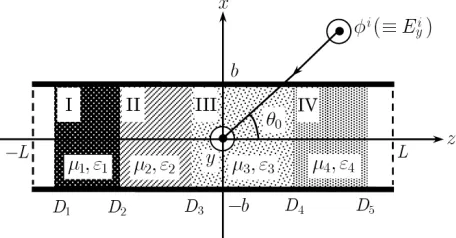
Figure 1. Geometry of the problem.

2. TRANSFORMED WAVE EQUATIONS

We consider the diffraction of an E-polarized plane wave by a finite parallel-plate waveguide with four-layer material loading as shown in Fig. 1, where −L < D1 < D2 < D3 < D4 < D5 < L and the E polarization implies that the incident electric field is parallel to the

m = 1,2,3, and 4, respectively. In view of the geometry and the characteristics of the incident field, this is a 2-D problem.

Define the total electric fieldφt(x, z)[≡E_yt(x, z)] by

φt(x, z) =φi(x, z) +φ(x, z), (1)

whereφi(x, z) is the incident field given by

φi(x, z) =e−ik(xsinθ0+zcosθ0) (2)

for 0 < θ0 < π/2 with k

≡ω(ε0µ0)1/2

being the free-space wavenumber. The total field φt_{(x, z) satisfies the 2-D Helmholtz} equation

∂2/∂x2+∂2/∂z2+µ(x, z)ε(x, z)k2φt(x, z) = 0, (3) where

µ(x, z) =

            

µ1(layer I)

µ2(layer II)

µ3(layer III)

µ4(layer IV) 1(otherwise)

, ε(x, z) =

            

ε1(layer I)

ε2(layer II)

ε3(layer III)

ε4(layer IV) 1(otherwise)

. (4)

Nonzero components of the total electromagnetic fields are derived from

E_yt, H_xt, H_zt =

φt, i ωµ0µ(x, z)

∂φt ∂z ,

i ωµ0µ(x, z)

∂φt ∂x

. (5)

We assume that the vacuum is slightly lossy as in k =k1+ik2 with 0 < k2 k1. The solution for realk is obtained by lettingk2 →+0 at the end of analysis. It follows from the radiation condition that the scattered field satisfies

φ(x, z) =O

e−k2|z|cosθ0

(6)

as|z| → ∞. We now define the Fourier transform of the scattered field

φ(x, z) with respect toz as

Φ(x, α) = (2π)−1/2

_∞

−∞φ(x, z)e

iαz_{dz, (7)}

complex α-plane. For convenience of analysis, we also introduce the Fourier integrals as

Φ_±(x, α) =±(2π)−1/2

_±∞

±L

φ(x, z)eiα(z∓L)dz, (8)

Φm(x, α) =

                  

(2π)−1/2

D1

−L

φt(x, z)eiαzdz, m= 1,

(2π)−1/2

Dm

Dm₋1

φt(x, z)eiαzdz, m= 2,3,4,5,

(2π)−1/2

L

D5

φt(x, z)eiαzdz, m= 6.

(9)

It is verified from the theory of Fourier integrals that Φ+(x, α) and Φ₋(x, α) are regular in the upper half-plane τ > −k2cosθ0 and the lower half-plane τ < k2cosθ0, respectively, whereas Φm(x, α) for

m = 1,2,3, . . ., 6 are entire functions. By using (8) and (9), we can express Φ(x, α) as

Φ(x, α) = Ψ(x, α) + Φ(1)(x, α), (10) where

Ψ(x, α) =e−iαLΨ₋(x, α) +eiαLΨ(+)(x, α), (11)

Φ(1)(x, α) = 6

m=1

Φm(x, α) (12)

with

Ψ₋(x, α) = Φ₋(x, α) +A e−

ikxsinθ0

α−kcosθ0

, (13)

Ψ₍₊₎(x, α) = Φ+(x, α)−B

e−ikxsinθ0

α−kcosθ0

, (14)

A= e

ikLcosθ0

(2π)1/2_i, B =

e−ikLcosθ0

(2π)1/2_i . (15) The parentheses in the subscript of Ψ₍₊₎(x, α) imply that Ψ₍₊₎(x, α) is regular inτ >−k2cosθ0 except for a simple pole atα=kcosθ0.

In order to derive transformed wave equations, we note that

and

∂2/∂x2+∂2/∂z2+K_m2 φt(x, z) = 0 (17) hold for unloaded and loaded regions, respectively, where Km = (µmεm)1/2kform= 1,2,3,4. For the region|x|> b, we can show by taking the Fourier transform of (16) and using (6) that

d2/dx2−γ2 Φ(x, z) = 0 (18) holds for any α in the strip |τ| < k2cosθ0, where γ = (α2 −k2)1/2 with Reγ >0. Equation (18) is the transformed wave equation for the region|x|> b.

The derivation of transformed wave equations for the region |x|< b is involved, since there are medium discontinuities across the surfaces at z = D1, D2, D3, D4, D5. We now multiply both sides of (17) by (2π)−1/2_eiαz _{and integrate with respect to z over the ranges} −∞ < z < D1 and D5 < z < ∞. Taking into account the boundary conditions for tangential electromagnetic fields at z = D1, D5, we derive by some manipulations that

d2/dx2−γ2 Φ1(x, α)+e−iαLΨ−(x, α)

=−eiαD1µ−₁1f1(x)−iαg1(x) (19)

forτ < k2cosθ0, and that

d2/dx2−γ2 Φ6(x, α)+e−iαLΨ(+)(x, α)

=eiαD5µ−₄1f5(x)−iαg5(x) (20)

forτ >−k2cosθ0 withα=kcosθ0, where

f1(x) = (2π)−1/2

∂φt(x, D1+ 0)

∂z , (21)

g1(x) = (2π)−1/2φt(x, D1), (22)

f5(x) = (2π)−1/2

∂φt_{(x, D} 5−0)

∂z , (23)

g5(x) = (2π)−1/2φt(x, D5). (24) Next we multiply both sides of (17) by (2π)−1/2_eiαz _{and integrate with} respect to z for D1 < z < D2, D2 < z < D3, D3 < z < D4, and

D4 < z < D5. This gives, after utilizing the boundary conditions for tangential electromagnetic fields atz=D1, D2, D3, D4, D5,

d2/dx2−Γ2₁ Φ2(x, α)

d2/dx2−Γ2₂ Φ3(x, α)

= eiαD2[f2(x)−iαg2(x)]−eiαD3[f3(x)−iαg3(x)], (26)

d2/dx2−Γ2₃ Φ4(x, α)

= eiαD3[(µ3/µ2)f3(x)−iαg3(x)]−eiαD4[f4(x)−iαg4(x)],(27)

d2/dx2−Γ2₄ Φ5(x, α)

= eiαD4[f4(x)−iαg4(x)]−eiαD5[f5(x)−iαg5(x)], (28) where Γm = (α2−Km2)1/2 with ReΓm>0 and

fm(x) = (2π)−1/2∂φ t_{(x, D}

m+ 0)

∂z , (29)

gm(x) = (2π)−1/2φt(x, Dm) (30) for m = 2,3,4. Equations (19), (20), and (25)–(28) are the transformed wave equations for the region|x|< b.

3. SIMULTANEOUS WIENER-HOPF EQUATIONS

First we shall solve the transformed wave Equations (18)–(20) and (25)–(28) to derive a scattered field representation in the Fourier transform domain. Using the boundary conditions for tangential electric fields across x=±b, the solution of (18) is expressed as

Φ(x, α) = Φ(b , α)e−γ(x−b), x≥b,

= Φ(−b , α)eγ(x+b), x≤ −b, (31) where we have used the following boundary conditions for tangential electric fields across x=±b:

Φ_±(±b+ 0, α) = Φ_±(±b−0, α)≡Φ_±(±b , α), (32) Φm(±b+ 0, α) = Φm(±b−0, α) = 0, m= 1,2,3, . . . ,6. (33) Equation (31) gives the scattered field representation for|x|> b.

The derivation of a field representation for the region |x| < b is complicated since the transformed wave equations involve the unknown inhomogeneous terms fm(x) and gm(x) for m = 1,2,3,4,5 . We expand these terms using the Fourier sine series as in

fm(x) = 1

b ∞

n=1

fmnsin

nπ

gm(x) = 1

b ∞

n=1

gmnsin

nπ

2b(x+b) (35)

for|x|< b, where

fmn =

b

−b

fm(x) sinnπ

2b(x+b)dx, (36) gmn =

b

−b

gm(x) sinnπ

2b(x+b)dx. (37)

The Fourier coefficientsfmnandgmnform= 1,2,3,4,5have various analytical properties which play a significant role in the subsequent analysis. These properties are discussed in detail in Appendix. Taking into account (34) and (35) and following a procedure similar to that employed in [20], we derive the solutions of (19), (20), and (25)–(28) with the result that

Φ1(x, α) +e−iαLΨ−(x, α)

= e−iαL

Ψ₋(b , α)sinhγ(x+b)

sinh 2γb −Ψ−(−b , α)

sinhγ(x−b) sinh 2γb

+e iαD1

b ∞

n=1

c−_1n(α)

α2_+γ2 n

sinnπ

2b(x+b), (38)

Φ6(x, α) +eiαLΨ(+)(x, α)

= eiαL

Ψ(+)(b , α)

sinhγ(x+b)

sinh 2γb −Ψ(+)(−b , α)

sinhγ(x−b) sinh 2γb

−eiαD5

b ∞

n=1

c−_5n(α)

α2_+γ2 n

sinnπ

2b(x+b), (39)

Φm(x, α) = −1

b ∞

n=1

eiαDm−1_c+

m−1, n(α)−eiαDmc−mn(α)

α2_{+ Γ}2 m−1, n

sinnπ

2b(x+b)

for m= 2,3,4,5, (40)

where

γn =

(nπ/2b)2−k21/2 forn≥1, (41) Γmn = (nπ/2b)2−K_m21/2 forn≥1, m= 1,2,3,4, (42)

c−_2n(α) = (µ1/µ2)f2n−iαg2n, c+2n(α) =f2n−iαg2n, (44)

c−_3n(α) = f3n−iαg3n, c+_3n(α) = (µ3/µ2)f3n−iαg3n, (45)

c+_4n(α) = f4n−iαg4n, c−4n(α) =f4n−iαg4n, (46)

c−_5n(α) = f5n−iαg5n, c+_5n(α) =µ−₄1f5n−iαg5n. (47) Substituting (38)–(40) into (10), the scattered field representation for the region|x|< b is derived.

Summarizing the above results, an explicit expression of Φ(x, α) is found to be

Φ(x, α) = Ψ(±b , α)e∓γ(x∓b) for x≷±b,

= Ψ(b , α)sinhγ(x+b)

sinh 2γb −Ψ(−b , α)

sinhγ(x−b) sinh 2γb

−1

b ∞

n=1

eiαD5_c+

5n(α)−eiαD1c−1n(α)

α2_+γ2 n

sinnπ

2b(x+b)

−1

b

4

m=1

∞

n=1

eiαDmc+_mm(α)−eiαDm+1c−_{m+1, n}(α)

α2_{+ Γ}2 mn

sinnπ

2b(x+b)

for |x|< b . (48) Equation (48) is the scattered field representation in the Fourier transform domain and holds in the strip|τ|< k2cosθ0.

Differentiating the field representation in (48) for x ≷ ±b with respect tox and settingx=±b±0, we obtain that

Φ(b+ 0, α) = −γΨ (−b , α), (49) Φ(−b−0, α) = −γΨ (−b , α), (50) where the prime denotes differentiation with respect to x. We also differentiate the field representation for |x| < b in (48) and set

x=±b∓0 in the results. Then it follows that Φ(b−0, α)=γΨ (b , α) coth 2γb−γΨ (−b , α) csch2γb

−1

b ∞

n=1

(−1)nnπ 2b

eiαD5_c+

5n(α)−eiαD1c−1n(α)

α2_+γ2 n

−1

b

4

m=1

∞

n=1

(−1)nnπ 2b

eiαDmc+_mn(α)−eiαDm+1c−_{m+1, n}(α)

α2_{+ Γ}2 mn

Φ(−b+ 0, α)=γΨ (b , α) csch2γb−γΨ (−b , α) coth 2γb

−1

b ∞

n=1

nπ

2b

eiαD5_c+

5n(α)−e−iαD1c−1n(α)

α2_+γ2 n

−1

b

4

m=1

∞

n=1

nπ

2b

eiαDmc+_mn(α)−eiαDm+1c−_{m+1, n}(α)

α2_{+ Γ}2 mn

. (52)

Subtracting (51) and (52) from (49) and (50), respectively and taking the sum and difference of the resultant equations, we obtain, after some manipulations, that

J₁d(α) = −e

−iαL_U

−(α) +eiαLU(+)(α)

M(α)

− ∞ n=1,odd

nπ b2

eiαD5c+_5n(α)−eiαD1c−_1n(α)

α2_+γ2 n

+ 4

m=1

eiαDm_c+

mn(α)−eiαDm+1c−m+1, n(α)

α2_{+ Γ}2 mn

, (53)

J₁s(α) = −e

−iαL_V

−(α) +eiαLV(+)(α)

N(α)

+

∞

n=2,even nπ

b2

eiαD5c+_5n(α)−eiαD1c−_1n(α)

α2_+γ2 n

+ 4

m=1

eiαDmc+_mn(α)−eiαDm+1c−_m+1,n(α)

α2_{+ Γ}2 mn

(54)

for|τ|< k2cosθ0, where

U₋(α) = Ψ₋(b , α) + Ψ₋(−b , α), (55)

U₍₊₎(α) = Ψ₍₊₎(b , α) + Ψ₍₊₎(−b , α), (56)

V₋(α) = Ψ₋(b , α)−Ψ₋(−b , α), (57)

V₍₊₎(α) = Ψ₍₊₎(b , α)−Ψ₍₊₎(−b , α), (58)

J₁d, s(α) = J1(b , α)∓J1(−b , α), (59)

J1(±b , α) = Φ(1)(±b±0, α)−Φ(1)(±b∓0, α), (60)

M(α) = e−

γb_coshγb

γ , N(α) =

e−γbsinhγb

Equations (53) and (54) are the simultaneous Wiener-Hopf equations satisfied by the unknown spectral functions, where the unknown Fourier coefficients are also involved.

4. FORMAL SOLUTION

The kernel functions M(α) and N(α) defined by (61) are factorized as [20]

M(α) =M+(α)M−(α), N(α) =N+(α)N−(α), (62)

whereM_±(α) andN_±(α) are the split functions given by

M+(α)[=M−(−α)]

= (coskb)1/2eiπ/4(k+α)−1/2exp{(iγb/π) ln[(α−γ)/k]} ·exp{(iαb/π)[1−C+ ln(π/2kb) +iπ/2]}

· ∞ n=1,odd

(1 +α/iγn)e2iαb/nπ, (63)

N+(α)[=N−(−α)]

= (sinkb/k)1/2exp{(iγb/π) ln[(α−γ)/k]} ·exp{(iαb/π)[1−C+ ln(2π/kb) +iπ/2]} · ∞

n=2,even

(1 +α/iγn)e2iαb/nπ (64)

withC(= 0.57721566. . .) being Euler’s constant. It is seem from (63) and (64) that M_±(α) and N_±(α) are regular and nonzero in τ ≷∓k2. We can also verify that

M_±(α)∼(∓2iα)−1/2, N_±(α)∼(∓2iα)−1/2 (65) as α → ∞ with τ ≷ ∓k2. Taking into account the edge condition, we can show that the unknown functions in (53) and (54) behave asymptotically as

U(+)(α)

U₋(α)

= O

α−3/2

, τ ≷∓k2cosθ0, (66)

e±iαLJ₁d(α) = O

α−1/2

for α → ∞. We multiply both sides of (53) by e±iαLM_±(α) and decompose the results using (65)–(67). This leads to

U₋(α)

M₋(α) − 1 2πi

C2

e2iβLU₍₊₎(β)

M₋(β) (β−α)dβ+

∞

n=1,odd nπ

2b

M+(iγn)

biγn(α−iγn) ·e−γn(L+D5)c+_5n(iγn)−e−γn(L+D1)c−_1n(iγn)

+ 4 m=1 ∞ n=1,odd nπ 2b

M+(iΓmn)

biΓmm(α−iΓmn)

·e−Γmn(L+D1)c+_mn(iΓmn)−e−Γmn(L+Dm+1)c−_{m+1, n}(iΓmn)

= 0,(68)

U₍₊₎(α)

M+(α) + 1

2πi

C1

e−2iβLU₋(β)

M+(β) (β−α)

dβ

+ 2Bcos (kbsinθ0)

M+(kcosθ0) (α−kcosθ0)−

∞

n=1,odd nπ

2b

M+(iγn)

biγn(α+iγn)

·e−γn(L−D5)c+_5n(−iγn)−e−γn(L−D1)c−_1n(−iγn)

− 4 m=1 ∞ n=1,odd nπ 2b

M+(iΓmn)

biΓmn(α+iΓmn)

·e−Γmn(L−D1)c+_mn(−iΓmn)−e−Γmn(L−Dm+1)c−m+1,n(−iΓmn)

= 0, (69)

whereC1 and C2 are the infinite integration paths running parallel to real axis in the β-plane, as shown in Fig. 2. Evaluating the integrals in (68) and (69) and arranging the results with the aid of (A4)–(A9) in Appendix, we derive that

U₋(α) = b1/2M₋(α)

Au

b(α−kcosθ0) +

Ju(1)(α)

b1/2

−∞ n=2

e−2γ2n−3(L+D1)_X−

2n−3anpnu−n

b(α−iγ2n−3) −∞

n=2

e−γ2n−3(2L+D1−D5)_Y−

2n₋3anpnu+n

b(α−iγ2n−3)

Figure 2. Integration paths C1 and C2 (0<|τ|< c < k2cosθ0).

U₍₊₎(α) = b1/2M+(α)

− Bu

b(α−kcosθ0) +J

(2) u (α)

b1/2

+

∞

n=2

e−2γ2n−3(L₋D5)_X+

2n−3anpnu+n

b(α+iγ2n₋3)

+

∞

n=2

e−γ2n−3(2L+D1−D5)_Y+

2n−3anpnu−n

b(α+iγ2n−3)

, (71)

where

X_n− = 1

G

e−2Γ1n(D2−D1)+ω1n µ1+

µ2Γ3n Γ2n

ξ1n

·

k µ1

+S4γnη1n

+

e−2Γ1n(D2−D1)+ω1n

·

µ1+

µ2Γ3n Γ2n ξ

1n

k µ1

+S4γnη1n

, (72)

Y_n− = 1

H

µ1 2µ2

+ Γ1n 2Γ2nτ

1n

R4

µ1

+γnS4 2 χn

·e−Γ1n(D2−D1)+eΓ1n(D2−D1)τ_1n

, (73)

X_n+ = 32

G µ2µ3

µ4

γnΓ4ne−Γ1n(D2−D1)

Y_n+ = (1/H)[µ4ρ43n(γnρ4n−2)

+Γ4nρ4n−µ4(Γ4n+γn)e−2Γ4n(D5−D4)], (75)

an= [(2n−3)π/2]2/biγ2n₋3, pn=b−1/2M+(iγ2n₋3), (76)

u−_n =b−1U₋(−iγ2n₋3), u+n =b−1U(+)(iγ2n₋3), (77)

J_u(1)(α) = 1

πi

k+i∞

k

e2iβL(β

2_−k2₎1/2_M

+(β)U(+)(β)

β−α dβ, (78)

J_u(2)(α) = 1

πi

k+i∞

k

e2iβL(β

2_−k2₎1/2_M

+(β)U−(−β)

β+α dβ, (79)

Au =

2b1/2Acos(kbsinθ0)

M₋(kcosθ0)

, Bu =

2b1/2Bcos(kbsinθ0)

M+(kcosθ0)

. (80)

A similar decomposition procedure can also be applied to (54). Omitting the details, we arrive at

V₋(α) = b1/2N₋(α)

− Av

b(α−kcosθ0) +J

(1) v (α)

b1/2

−

∞

n=2

e−2γ2n−2(L+D1)_X−

2n−2bnqnv−n

b(α−iγ2n₋2) −∞

n=2

e−γ2n−2(2L+D1−D5)_Y−

2n−2bnqnv+n

b(α−iγ2n−2)

, (81)

V₍₊₎(α) = b1/2N+(α)

Bv

b(α−kcosθ0) +J

(2) v (α)

b1/2

+

∞

n=2

e−2γ2n−2(L−D5)_X+

2n−2bnqnv+n

b(α+iγ2n−2)

+

∞

n=2

e−γ2n−2(2L+D1−D5)_Y+

2n−2bnqnvn−

b(α+iγ2n−2)

, (82)

where

bn= [(n−1)π]2/biγ2n₋2, qn=b−1/2N+(iγ2n₋2), (83)

J_v(1)(α) = 1

πi

k+i_∞

k

e2iβL(β

2_−k2₎1/2_N

+(β)V(+)(β)

β−α dβ, (85)

J_v(2)(α) = 1

πi

k+i∞

k

e2iβL(β

2_−k2₎1/2_N

+(β)V−(−β)

β+α dβ, (86)

Av =

2ib1/2Asin(kbsinθ0)

N₋(kcosθ0)

, Bv=

2ib1/2Bsin(kbsinθ0)

N+(kcosθ0)

. (87)

Several coefficients appearing in (72)–(75) are defined in Appendix. Equations (70), (71) and (81), (82) are the exact solutions of the Wiener-Hopf equations (53) and (54), respectively, but they are formal since the infinite series with the unknown coefficientsu±_n andv_n±forn= 2,3,4, . . . as well as the branch-cut integralsJu(1),(2)(α) andJv(1),(2)(α) with unknown integrands U₋(α), U₍₊₎(α), V₋(α), and V₍₊₎(α) are involved. Therefore, it is required to develop approximation procedures for an explicit solution.

5. APPROXIMATE SOLUTION

In this section, we shall evaluate the infinite series and branch-cut integrals occurring in the formal solutions to derive approximate solutions of the Wiener-Hopf equations. To this end, we can apply the method established in [19] for the analysis of the diffraction by a parallel-plate waveguide cavity.

First we shall derive an approximate expression ofU₋(α) defined by (70). Assuming that the waveguide length 2L is large compared with the wavelength and applying the method in [19], the branch-cut integralJu(1)(α) defined by (78) can be expanded asymptotically as

J_u(1)(α)∼J_u(11)(α) +J_u(12)(α) (88) forkL→ ∞, where

J_u(11)(α) =b1/2a1p1

u+₁ +2Bcos(kbsinθ0)

kb(1−cosθ0)

ξ(−α), (89)

J_u(12)(α) = 2Lb−1/2a1p1Bcos(kbsinθ0)

ξ(−α)−ξ(−kcosθ0) (−α+kcosθ0)L

(90)

with

a1 = kb, p1 =b−1/2M+(k), u+1 =b−1U(+)(k), (91)

ξ(α) = e

i(2kL−π/4)

In (92) Γ1(·,·) is the generalized gamma function [27] defined by

Γm(u, v) =

_∞

0

tu−1e−t

(t+v)dt (93)

for Reu >0, |v|>0, |argv|< π, and positive integerm.

Using (66), it is found that the coefficients u±_n defined by (77) show the asymptotic behavior

u−_n ∼21/2K_u(1)(bγ2n−3)−3/2, u+n ∼21/2Ku(2)(bγ2n−3)−3/2 (94) as n → ∞, where Ku(1) and Ku(2) are unknown constants. Taking a large positive integer N and replacing u±_n for n ≥ N by their asymptotic behavior (94), each infinite series occurring in (70) can be approximated in reasonable accuracy by the sum of the finite series containing N −2 unknowns and the infinite series with one unknown constant. This procedure yields an accurate approximate expression of the original infinite series since the edge condition is taken into account explicitly. Thus we arrive at the approximate expression of (70) with the result that

U₋(α) ≈ b1/2M₋(α)

Au

b(α−kcosθ0) +a1p1

u+₁ +2Bcos (kbsinθ0)

kb(1−cosθ0)

ξ(−α)

+2LB

b cos (kbsinθ0)

ξ(−α)−ξ(−kcosθ0) (−α+kcosθ0)L

− N₋1

n=2

anpnX2n−−3e−2γ2n−3(L+D1)u−n

b(α−iγ2n₋3) −

N−1

n=2

anpnY2n−₋3e−γ2n−3(2L+D1−D5)u+n

b(α−iγ2n−3) −K_u(1)

∞

n=N

anX2n−−3(bγ2n−3)−2e−2γ2n−3(L+D1)

b(α−iγ2n−3) −K_u(2)

∞

n=N

anY2n−−3(bγ2n−3)−2e−γ2n−3(2L+D1−D5)

b(α−iγ2n−3)

(95)

A similar procedure can also be applied to derive approximate expressions of (71), (81), and (82). This leads to

U₍₊₎(α) ≈ b1/2M+(α)

− Bu

b(α−kcosθ0) +a1p1

u−₁ +2Acos (kbsinθ0)

kb(1 + cosθ0)

ξ(α)

+2LA

b cos (kbsinθ0)

ξ(α)−ξ(kcosθ0) (α−kcosθ0)L

− N−1

n=2

anpnX2n+−3e−2γ2n−3(L−D5)u+n

b(α+iγ2n₋3)

+ N−1

n=2

anpnY2n−₋3e−γ2n−3(2L+D1−D5)u−n

b(α−iγ2n−3)

+K_u(2) ∞

n=N

anX2n+−3(bγ2n−3)−2e−2γ2n−3(L−D5)

b(α+iγ2n−3)

+K_u(1) ∞

n=N

anY2n+−3(bγ2n−3)−2e−γ2n−3(2L+D1−D5)

b(α+iγ2n₋3)

, (96)

V₋(α) ≈ b1/2N₋(α)

− Av

b(α−kcosθ0) +b1q1

v₁+−2iBsin (kbsinθ0) kb(1−cosθ0)

ξ(−α) −2iLB

b sin (kbsinθ0)

ξ(−α)−ξ(−kcosθ0) (−α+kcosθ0)L

− N−1

n=2

bnqnX2n−−2e−2γ2n−2(L+D1)vn−

b(α−iγ2n−2) −

N₋1

n=2

bnqnY2n−−2e−γ2n−2(2L+D1−D5)v+n

b(α−iγ2n₋2) −K_v(1)

∞

n=N

bnX2n−₋2(bγ2n−2)−2e−2γ2n−2(L+D1)

b(α−iγ2n−2) −K_v(2)

∞

n=N

bnY_2n−₋₂(bγ2n₋2)−2e−γ2n−2(2L+D1−D5)

b(α−iγ2n−2)

V(+)(α) ≈ b1/2N+(α)

Bv

b(α−kcosθ0) +b1q1

v₁−+2iAsin (kbsinθ0)

kb(1 + cosθ0)

ξ(α)

−2iLA

b sin (kbsinθ0)

ξ(α)−ξ(kcosθ0) (α−kcosθ0)L

+ N−1

n=2

bnqnX_2n+₋₂e−2γ2n−2(L−D5)vn+

b(α+iγ2n−2)

+ N−1

n=2

bnqnY2n+−2e−γ2n−2(2L+D1−D5)vn−

b(α+iγ2n₋2)

+K_v(2) ∞

n=N

bnX2n−−2(bγ2n−2)−2e−2γ2n−2(L−D5)

b(α+iγ2n−2)

+K_v(1) ∞

n=N

bnY2n+₋2(bγ2n−2)−2e−γ2n−2(2L+D1−D5)

b(α+iγ2n−2)

(98)

for largeN and |k|L, where

b1 =kb, q1 =b−1/2N+(k), (99)

u−₁ =b−1U₋(−k); v₁−=b−1V₋(−k), v+₁ =b−1V₍₊₎(k). (100) In the derivation of (97) and (98), we have used the edge condition

v_n−∼21/2K_v(1)(bγ2n₋2)−3/2, u+n ∼21/2Kv(2)(bγ2n₋2)−3/2 (101) forn→ ∞, whereKv(1) and Kv(2) are unknown constants.

Equations (95), (96) and (97), (98) are approximate solutions to the Wiener-Hopf Equations (53) and (54), respectively, and they are valid for large positive integer N and large |k|L. The unknown u±_n

and v±_n forn= 1,2, . . . , N−1 and Ku(1),(2), Kv(1),(2) in (95)–(98) are determined with high accuracy by solving appropriate 2N×2N matrix equations numerically.

6. SCATTERED FIELD

The scattered field can be derived by taking the inverse Fourier transform of (48) according to the formula

φ(x, z) = (2π)−1/2

_∞+ic

−∞+ic

where |c| < k2cosθ0. First let us consider the field inside the waveguide. Substituting the field representation for |x| < b in (48) into (102) and evaluating the resultant integral, we find from (1) that the total field for the region inside the waveguide is expressed in terms of the TE modes and takes the form

φt(x, z) =

∞

n=1

T_Ln+eγn(z−D1)−T_Ln−e−γn(z−D1)

sinnπ

2b(x+b)

for −L < z < D1, =

∞

n=1

T_mn+ eΓm(z−Dm)−T_mn− e−Γm(z−Dm)

sinnπ

2b(x+b)

forDm < z < Dm+1, m= 1,2,3,4,

=

∞

n=1

T_Rn+ eγn(z−D5)−T_Rn− e−γn(z−D5)

sinnπ

2b(x+b)

forD5 < z < L, (103) where

T_Ln− = −χne−γn(L+D1)U−(−iγn) for oddn,

= χne−γn(L+D1)V−(−iγn) for evenn, (104)

T_Ln+ = −χn

X_n−e−γn(L+D1)U₋(−iγn) +Yn−e−γn(L−D5)U(+)(iγn)

for oddn,

= χn

X_n−e−γn(L+D1)V₋(−iγn) +Yn−e−γn(L−D5)V(+)(iγn)

for evenn, (105)

T_Rn− = χn

Y_n+e−γn(L+D1)U₋(−iγn) +Xn−e−γn(L−D5)U(+)(iγn)

for oddn,

= −χn

Y_n+e−γn(L+D1)V₋(−iγn) +Xn−e−γn(L−D5)V(+)(iγn)

for evenn, (106)

T_Rn+ = χne−γn(L−D5)U(+)(iγn) for oddn,

= −χne−γn(L−D5)V(+)(iγn) for evenn, (107)

T_mn− = −Kmn

R−_mnU₋(−iγn) +Smn− U(+)(iγn)

for oddn(m= 1,2,3,4),

= Kmn

R−_mnV₋(−iγn) +S_mn− V(+)(iγn)

T_mn+ = −Kmn

R+_mnU₋(−iγn) +Smn+ U(+)(iγn)

for oddn(m= 1,2,3,4),

= Kmn

R+_mnV₋(−iγn) +S_mn+ V(+)(iγn)

for evenn(m= 1,2,3,4), (109)

R−_1n = P1n−Γ1nR1n, R1n+ = (µ1/µ2)P2n+ Γ1nR2n,

S_1n− = Q1n−Γ1nS1n, S1n+ = (µ1/µ2)Q2n+ Γ1nS2n, (110)

R−_2n = P2n−Γ2nR2n, R+2n=P3n+ Γ2nR3n, (111)

S_2n− = Q2n−Γ2nS2n, S_2n+ =Q3n+ Γ2nS3n, (112)

R−_3n = (µ3/µ2)P3n−Γ3nR3n, R3n+ =P4n+ Γ3nR4n, (113)

S_3n− = (µ3/µ2)Q3n−Γ3nS3n, S3n+ =Q4n+ Γ3nS4n, (114)

R−_4n = (µ4/µ3)P4n−Γ4nR4n, R4n− = (µ4/µ3)P4n+ Γ4nR4n, (115)

S_4n− = (µ4/µ3)Q4n−Γ4nS4n, S_4n+ = (µ4/µ3)Q4n+ Γ4nR4n, (116)

χn =

_π

2

1/2 _nπ 2b2_γ n

;Kmn =

_π

2

1/2 _nπ

2b2_Γmnform= 1,2,3,4,(117) In (110)–(114), the definition of Pmn, Qmn, Rmn, and Smn for

m= 1,2,3,4 is given in Appendix.

Next we shall consider the field outside the waveguide and derive the scattered far field. Substituting the field representation for|x|> b

in (48) into (102) and evaluating the resultant integral asymptotically with the aid of the saddle point method, we obtain a far field expression

φ(ρ, θ)∼Ψ(±b,−kcosθ)ksinθe±ikbsinθe

i(kρ−π/4)

(kρ)1/2 (118)

for x ≷ ±b as kρ → ∞, where (ρ, θ) is the cylindrical coordinate defined by x=ρsinθ, z=ρcosθ for 0<|θ|< π. In (119), Ψ(±b , α) is expressed as

Ψ(±b , α) =e−iαLU−(α)±V−(α)

2 +e

iαLU(+)(α)±V(+)(α)

2 (119)

7. NUMERICAL RESULTS AND DISCUSSION

In this section, we shall show representative numerical examples of the RCS for various physical parameters to discuss the far field scattering characteristics of the waveguide in detail. Numerical results presented below are based on the use of the scattered far field expression as given by (119) together with (120). We have used the approximate expressions as derived in (95)–(98) for computing the functions U₋(α), U(+)(α), V−(α), and V(+)(α) involved in (120). As has been mentioned at the end of Section 5, we need to solve the two sets of 2N ×2N matrix equations numerically for obtaining all the physical quantities. According to the theory of the Wiener-Hopf technique, convergence of the approximate solutions obtained in Section 5is very fast for a small waveguide aperture 2b, since we then do not require large N in numerical computation. In order for the approximate solutions to be reasonably accurate, however, some large N is needed with an increase of 2b. By careful numerical experimentation, we have verified that sufficiently accurate results can be obtained by choosing N ≥2kb/πin (95)–(98).

We shall now investigate the scattering mechanism via numerical results of the monostatic and bistatic RCS for various physical parameters. Since the problem considered here is of the two-dimensional scattering, the RCS per unit length is defined by

σ = lim ρ_→∞

2πρ|φ|2/φi2

. (120)

For realk, (121) is simplified by using (2) and (118) as

σ =λ|Ψ(±b,−kcosθ)ksinθ|2, θ≷0, (121) whereλis the free-space wavelength.

Figures 3 and 4 show the monostatic RCS σ/λ as a function of incident angleθ0where the values ofσ/λare plotted in decibels [dB] by computing 10 log₁₀σ/λ. The waveguide structure is symmetric along thez-axis so that we have presented the RCS data only for the range 0◦ ≤θ0≤180◦. In order to investigate the scattering mechanism over a broad frequency range, we have carried out numerical computation for three typical values of the normalized waveguide aperture width

kb= 3.14, 15.7, and 31.4, which correspond to low, medium, and high frequencies, respectively. For a fixed kb, the ratio of the waveguide length 2L to the waveguide aperture width 2b has been chosen as

Figure 3a. Monostatic RCS σ/λ [dB] for L/b = 1.0, kb = 3.14. -·-·-·-·-·-·- empty waveguide (layers I-IV: vacuum). : cavity with no loading (layer I: perfect conductor; layers II-IV: vacuum; tL = 0.6L, tPEC = 0.4L, tR = L). : cavity with two-layer

loading (layer I: perfect conductor; layer II:ε2= 3.14+i10.0, µ2 = 1.0;

layer III:ε3 = 1.6+i0.9, µ3= 1.0; layer IV: vacuum;tL= 0.6L, tPEC =

0.4L, tR =L, t2layer = 0.4L). ——–: cavity with three-layer loading

(layer I: perfect conductor; layers II-IV: Emerson & Cuming AN-73; tL= 0.6L, tPEC= 0.4L, tR=L, t3layer= 0.6L).

Figure 3c. Monostatic RCSσ/λ[dB] forL/b= 1.0,kb= 31.4. Other particulars are the same as in Fig. 3a.

Figure 4a. Monostatic RCSσ/λ[dB] forL/b= 3.0,kb= 3.14. Other particulars are the same as in Fig. 3a.

and right (D2 < z < L) sides of the waveguide. We have chosen the depth of the left and right cavities as tL(= D1 +L) = 0.6L and

Figure 4b. Monostatic RCSσ/λ[dB] forL/b= 3.0,kb= 15.7.Other particulars are the same as in Fig. 3a.

Figure 4c. Monostatic RCSσ/λ[dB] forL/b= 3.0,kb= 31.4. Other particulars are the same as in Fig. 3a.

Cuming AN-73 [2] with the material constants beingε2 = 3.14 +i10.0,

t2layer = 0.4L and t3layer = 0.6L, respectively. In addition, the results for an empty parallel-plate waveguide (εn= µn = 1.0, n= 1,2,3,4) have also been plotted for comparison.

It is seen from Figs. 3 and 4 that the monostatic RCS exhibits sharp peaks at θ0 = 90◦, which correspond to the specular reflection from the upper waveguide plate at x = b. Due to the geometrical symmetry, the RCS curves for the parallel-plate waveguide with no material loading are symmetrical around the main lobe direction at

θ0 = 90◦. For fairly large square-shape cavities (L/b = 1.0) with no material loading, the RCS takes close values at θ0 = 0◦,90◦,180◦ as seen from Figs. 3(b) and 3(c), since contributions to the backscattered far field at high frequencies mainly come from the reflected waves from the perfectly conducting surfaces atx=b and z=D1, D2.

We find from the four curves in Figs. 3 and 4 that the RCS characteristics of all the waveguide geometries for fixed kb and L/b

show close features near the main lobe direction 80◦< θ0 <100◦. This is because main contributions to the backscattered far field arise from exterior features of the waveguide, not depending on features inside the waveguide. We also notice from the results of the three cavities for fixedkb and L/b that the RCS characteristics for 90◦< θ0 <180◦ are nearly identical to each other, since the cavity formed at the right side of the waveguide is then invisible from the incident direction and the backscattered far field is not affected by the interior geometries of the right cavity.

We now investigate the effect of material loading inside the right cavity. For the cavity with no material loading, the RCS shows large values over the range 0◦ < θ0 < 80◦ due to the interior irradiation, whereas the irradiation is reduced for the case of material loading. By comparing the RCS results for material-loaded cavities between the two-layer case and the three-layer case (Emerson & Coming AN-73), we see better RCS reduction in the case of the cavity with three-layer loading for all chosenkbandL/b. Incidentally, the empty parallel-plate waveguide for largekb(= 15.7,31.4) shows very low RCS values except in the neighborhood ofθ0 = 90◦ because only the edge-diffracted fields contribute to the backscattered far field.

Figures 5and 6 show the bistatic RCSσ/λ [dB] as a function of observation angle θ, where the incidence angle is chosen as θ0 = 45◦, and other parameters are the same as in Figs. 3 and 4. From Figs. 5and 6, it is found that the bistatic RCS shows noticeable peaks atθ=−135◦ and θ= 135◦ for all the four waveguide geometries, which correspond to the incident and reflected shadow boundaries, respectively. It is also seen that, for L/b = 1.0 and kb= 15.7,31.4, the peak RCS values at

than those for the other three geometries (cavities with and without material loading) as seen from Figs. 5(b) and 5(c). This is because contributions to the scattered far field along theθ= 135◦ direction for the empty parallel-plate waveguide arise due to the specular reflection

Figure 5a. Bistatic RCSσ/λ[dB] forL/b= 1.0,kb= 3.14,θ0 = 45◦.

-·-·-·-·-·-·- empty waveguide (layers I-IV: vacuum). : cavity with no loading (layer I: perfect conductor; layers II-IV: vacuum; tL = 0.6L, tPEC = 0.4L, tR = L). : cavity with two-layer

loading (layer I: perfect conductor; layer II:ε2= 3.14+i10.0, µ2 = 1.0;

layer III:ε3 = 1.6+i0.9, µ3= 1.0; layer IV: vacuum;tL= 0.6L, tPEC =

0.4L, tR =L, t2layer = 0.4L). ——–: cavity with three-layer loading

(layer I: perfect conductor; layers II-IV: Emerson & Cuming AN-73; tL= 0.6L, tPEC= 0.4L, tR=L, t3layer= 0.6L).

Figure 5b. Bistatic RCSσ/λ[dB] forL/b= 1.0,kb= 15.7,θ0 = 45◦.

Figure 5c. Bistatic RCSσ/λ[dB] forL/b= 1.0,kb= 31.4,θ0 = 45◦.

Other particulars are the same as in Fig. 5a.

Figure 6a. Bistatic RCSσ/λ[dB] forL/b= 3.0,kb= 3.14,θ0 = 45◦.

Other particulars are the same as in Fig. 5a.

from both the upper and lower plates, but the reflected waves from the lower plate do not contribute to the bistatic scattering in the case of cavities. By comparing Figs. 5and 6, we find that the peaks at

θ=±135◦ become sharper with an increase of L/b as expected. It is also observed that, when L/b = 3.0, the RCS of the parallel-plate waveguide and the cavities at θ = 135◦ shows close values as the reflected waves from the lower plate then do not contribute much to the scattered far field unlike the case ofL/b = 1.0. The other feature in Figs. 5and 6 is that there are some peaks in the neighborhood of

Figure 6b. Bistatic RCSσ/λ[dB] forL/b= 3.0,kb= 15.7,θ0 = 45◦.

Other particulars are the same as in Fig. 5a.

Figure 6c. Bistatic RCSσ/λ[dB] forL/b= 3.0,kb= 31.4,θ0 = 45◦.

Other particulars are the same as in Fig. 5a.

8. CONCLUSIONS

In this paper, we have considered a finite parallel-plate waveguide with four-layer loading as a generalization to the geometry treated in our previous papers [24, 25], and analyzed rigorously the E-polarized plane wave diffraction by means of the Wiener-Hopf technique. We have obtained exact and approximate solutions to the Wiener-Hopf equations. Since the approximate solution has been derived on the basis of a rigorous asymptotics, our final results are valid for the waveguide length large compared with the incident wavelength. We have presented illustrative numerical examples of the monostatic and bistatic RCS for various physical parameters to discuss the far field scattering characteristics in detail. In particular, it has been shown that the four-layer material loading gives rise to a better RCS reduction compared with the three-layer case analyzed in our previous papers. The results can be used as a reference solution for validating more general but approximate approaches. A similar Wiener-Hopf analysis for the case of the H-polarized plane wave incidence is carried out in the companion paper [26].

ACKNOWLEDGMENT

This work was supported in part by the Institute of Science and Engineering, Chuo University.

APPENDIX A. ANALYTICAL PROPERTIES OF THE FOURIER COEFFICIENTS

This appendix concerns the derivation of important formulas for the Fourier coefficients, which play an essential role in solving the Wiener-Hopf equations. We first note that Ψ₋(x, α) is regular inτ < k2cosθ0 (see (8) and (13)) and Ψ₍₊₎(x, α) is regular in τ > −k2cosθ0 except for a simple pole atα=kcosθ0 (see (8) and (14)), whereas Φm(x, α) form= 1,2,3, . . . ,6 are entire functions (see (9)). Hence, we deduce that

lim

α→−iγn(α+iγn)

Φ1(x, α) +e−iαLΨ−(x, α)

= 0, (A1) lim

α_→iγn(α−iγn)

Φ6(x, α) +eiαLΨ(+)(x, α)

= 0, (A2) lim

for n = 1,2,3, . . . Substituting (38), (39), and (40) into (A1), (A2), and (A3), respectively, we derive, after some manipulations, that

c−_1n(−iγn) = −nπ 2be

−γn(L+D1)_U

−(−iγn) for oddn,

= nπ 2be

−γn(L+D1)_V

−(−iγn) for evenn, (A4)

c+_5n(iγn) =

nπ

2be

−γn(L−D5)_U

(+)(iγn) for oddn, = −nπ

2be

−γn(L−D5)_V

(+)(iγn) for evenn, (A5)

c+_mn(iΓmn)−e−Γmn(Dm+1−Dm)c−m+1, n(iΓmn) = 0

for n= 1,2,3, . . . , (A6)

e−Γmn(Dm+1−Dm)c+_mn(−iΓmn)−c−m+1, n(−iΓmn) = 0

for n= 1,2,3, . . . . (A7) Equations (A4)–(A7) constitute a system of simultaneous algebraic equations, which relates the Fourier coefficientsfmn andgmn for m = 1,2,3,4,5with the functions U₋(α), U₍₊₎(α), V₋(α), and

V₍₊₎(α). Solving these equations forfmnandgmnform= 1,2,3,4,5, we are led to

fmn=−

nπ

2b

e−γn(L+D1)PmnU−(−iγn)+e−γn(L−D5)QmnU(+)(iγn)

for oddn,

=nπ 2b

e−γn(L+D1)PmnV−(−iγn) +e−γn(L−D5)QmnV(+)(iγn)

for evenn,(A8)

gmn=−

nπ

2b

e−γn(L+D1)RmnU−(−iγn) +e−γn(L−D5)SmnU(+)(iγn)

for oddn,

=nπ 2b

e−γn(L+D1)RmnV₋(−iγn) +e−γn(L−D5)SmnV(+)(iγn)

for evenn, (A9) where

P5n = (16/G)µ2µ3γnΓ4ne−Γ4n(D5−D4)e−Γ3n(D4−D3)

·e−Γ2n(D3−D2)e−Γ1n(D2−D1), (A10)

Q5n = (1/H)

γnµ24ρ43n(ρ4n−1) +µ4γn

ρ43nρ4n−e−2Γ4n(D5−D4)

R5n = (16/G)(µ2µ3/µ4)γnΓ4ne−Γ4n(D5−D4)

·e−Γ3n(D4−D3)e−Γ2n(D3−D2)e−Γ1n(D2−D1), (A12)

S5n = −(1/H)µ4[ρ43n−e−2Γ4n(D5−D4)], (A13)

P4n = (8/G)µ2Γ4n(µ4γn+ Γ4n)e−Γ3n(D4−D3) ·e−Γ2n(D3−D2)e−Γ1n(D2−D1)

e−2Γ4n(D5−D4)+ρ4n

, (A14)

Q4n =− 1

H

µ4

µ3

Γ4n(ρ43n+µ4)e−Γ4n(D5−D4)

−µ4ρ43n(ρ4n+ 1)

γn

µ2₄

2µ3

δ4n+ Γ4n

eΓ4n(D5−D4)

, (A15)

R4n = (8/G)(µ2µ3/µ4)(µ4γn+ Γ4n)e−Γ3n(D4−D3)

·e−Γ2n(D3−D2)e−Γ1n(D2−D1)[e−2Γ4n(D5−D4)−ρ4n], (A16)

S4n = 1

H

µ4(ρ43n−1)e−Γ4n(D5−D4)−

µ4 2 ρ43n ·(ρ4n+ 1)

γn

Γ4nµ4δ4n+ 1

eΓ4n(D5−D4)

, (A17)

P3n = 1

G

4µ2 2

µ3µ4

(µ4γn+ Γ4n)

µ3Γ3n

µ4

+ Γ4n

e−Γ2n(D3−D2)

·e−Γ1n(D2−D1)

e−2Γ4n(D5−D4)

e−2Γ3n(D4−D3)+ρ3n

+ρ3nρ4n

e−2Γ3n(D4−D3)+ 1

, (A18)

Q3n = 1

H

µ2I 2µ3

e−Γ4n(D5−D4)

x3ne−Γ3n(D4−D3)−eΓ3n(D4−D3)

+µ2J 2µ3

ρ4n+1eΓ4n(D5−D4)

y3ne−Γ3n(D4−D3)+eΓ3n(D4−D3)

, (A19)

R3n = (1/G)((4µ2/Γ3n)(µ4γn+Γ4n) [(µ3Γ3n/µ4)+Γ4n] ·e−Γ2n(D3−D2)e−Γ1n(D2−D1)

e−2Γ4n(D5−D4)

·e−2Γ3n(D4−D3)−ρ3n

+ρ4n

ρ3ne−2Γ2n(D4−D3)−1

, (A20)

S3n = 1

H

I

2Γ3n

eΓ4n(D5−D4)

x3ne−Γ3n(D4−D3)+eΓ3n(D4−D3)

+ J 2Γ3n

(ρ4n+ 1)eΓ4n(D5−D4)

·y3ne−Γ3n(D4−D3)−e−Γ3n(D4−D3)

P2n = 2µ2

G (µ4γn+ Γ4n)

µ3Γ3n

µ4

+ Γ4n

(R1+R2), (A22)

Q2n = (1/4H)(R3+R4), (A23)

R2n = 2µ2

G (µ4γn+Γ4n)

µ3Γ3n

µ4

+Γ4n

e−Γ1n(D2−D1)(S1+S2),(A24)

S2n = (1/4H)(S3+S4), (A25)

P1n = 1

G

(µ4γn+ Γ4n)

µ3Γ3n

µ4

+ Γ4n

·R1

µ1+

µ2Γ3n

Γ2n ξ1n e

−2Γ1n(D2−D1)_+ω 1n

+R2

µ1+

µ2Γ3n Γ2n ξ

1n e−2Γbn(D2−D1)+ω1n

, (A26)

Q1n= 1

H

R3

µ1 2µ2

+ Γ1n 2Γ2n

τ1n e−Γ1n(D2−D1)+eΓ1n(D2−D1)τ1n

+R4

µ1 2µ2

+ Γ1n 2Γ2n

τ_1n

e−Γ1n(D2−D1)+eΓ1n(D2−D1)τ1n

,(A27)

R1n = 1

G

S1

2Γ1n(µ4γn+ Γ4n)

µ3Γ3n

µ4

+ Γ4n

·

µ1+

µ3Γ3n

µ2

ξ1n e−2Γ1n(D2−D1)−ω1n

+S2

µ1+

µ3Γ3n

µ2

ξ_1n e−2Γ1n(D2−D1)−ω_1n

, (A28)

S1n= 1 4H S3 µ1 µ2

+τ1nΓ1n Γ2n

e−Γ1n(D2−D1)+eΓ1n(D2−D1)τ1n

+S4

µ1

µ2

+τ1n Γ1n Γ2n

e−Γ1n(D2−D1)+eΓ1n(D2−D1)τ_1n

,(A29)

G = (µ1γn+Γ1n)(µ4γn+Γ1n)

µ3

µ4

+δ32nΓ4n Γ3n

µ2

µ1

+δ1nΓ2n Γ1n

·ρ43nρ4n−e−2Γ4n(D5−D4) ρ32n+e−2Γ3n(D4−D3)

·ρ21n+e−2Γ2n(D3−D2) 1 +e−2Γ1n(D2−D1)ρ1n

, (A30)

H = (µ4γ4n+ Γ4n)

ρ43nρ4n−e−2Γ4n(D5−D4)

, (A31)

I = [µ4Γ3n(ρ43n−1) + Γ4n(µ4/µ3) (ρ4n+µ4)]−1, (A32)

J =

µ4ρ43n

µ2 4δ4nγn

2µ3

+Γ4n

+µ4

2 Γ3nρ43n

µ4δ4nγn Γ4n +1

₋1