Volume 5(3)2015, pp. 40-51
40
THE EVALUATION OF LOGISTICS-ORIENTED ECONOMIC DEVELOPMENT
LEVEL BASED ON PRINCIPAL COMPONENT ANALYSIS AND CLUSTER
ANALYSIS: THE CASE OF GUANGDONG PROVINCE
Xia Pan
Lingnan College, Sun Yat-sen University, Guangzhou, China
Jeffrey E. Jarrett
Faculty of Management Science and Finance, University Of Rhode Island, Kingston, RI, USA
Abstract
This paper tries to cluster the cities in Guangdong Province, China according to their economic development levels. We intentionally separate a group of indicators for logistics and transportation development levels, therefore, the clustering results can be viewed as in accordance with logistics-oriented economic development levels. Before the clustering, we use principal component analysis to reduce the number of dimensions. The results of the final categories are consistent with what many people perceived about the clusters according to the city’s economic development levels, as well as how much the cities' logistics is developed. This findings provide the business and public administration decision makers the references in their decisions on developing the respective city's logistics and transportation.
Keywords: Logistics oriented economic development, cluster analysis, Pseudo-t2 statistics, component matrix
1. INTRODUCTION
1The objective of this study is to apply a methodology for improving economic development in a region involving a logistics model to efficiently move product from place to place. The result is to improve by using the logistics system to enable the supply chain environment to be sustained, improved and to run efficiently the overall performance of urban freight systems. This contribution appears to be an attempt to develop a framework for capturing the sustainability (economic, social, environmental) aspects of shipping freight. This attempt is also a challenge, considering that economic and environmental issues are quite difficult to measure, as opposed to physical phenomena measured through mechanical devices. This subject is crucial for the improvement of transportation planning in emerging nations. The evaluation of freight issues and policies would benefit from the existence of globally accepted methodologies for handling issues in the supply chain.
Ramanathan (2001) studied how to design a system for prioritizing their environment management plan and strengthen decisions for allocation of a budget. This budget plan is designed to producemethods for mitigating adverse socio-economic impacts. Later, Allen et al. (2003) and Anderson et al. (2005) laid the groundwork for reflecting the sustainability of urban distribution operations. Methodological problems in developing nations to determine the appropriate models and
Corresponding author's Name: Jeffrey E. Jarrett
Email address: [email protected]
Asian Journal of Empirical Research
http://www.aessweb.com/journals/5004
41
tools for the analysis, planning and operations of a system to measure freight transportation in congested areas was studied by Crainic et al. (2004). Others [May et al. (2006, 2008), Patier and Brown (2010), Filippi et al. (2010) and Betanzo-Quezada (2012)] proceeded to raise additional questions concerning assessments concerning urban freight. Based on these previous studies, we approach the problems of freight so that decision makers can see better methods and understanding of the problem.
2. RESEARCH METHODS
2.1. Principal component analysis
We convert a set of indictors into a few comprehensive variables, eliminating the correlation amount the original indictors and replacing the original multiple indicators with several comprehensive ones. Second, we determine several predictor (explanatory) variables which best explain the original information from numerous observations. The purpose is to reduce the dimensionality of multi-dimensional variables, simplify the data structures, and result in a convenient method convenient for problem resolving.
2.2. Cluster analysis
Cluster analysis achieves grouping a set of objects by multivariate statistical methods according to its object features. The procedure creates groups consisting of observations by their features and aims to achieve that sample observations in the same group are more similar to each other than to those in other groups. In this study, we arrive at a sample matrix by the q top primary component which results from the principal component analysis method. The process involves finding the Euclidean distance between samples, as well as determining class average (mean) method between classes. Last, by using Pseudo-t2 Statistics, one determines the cluster number (Vizirgiannis et al.,
2003).
2.3. Research framework
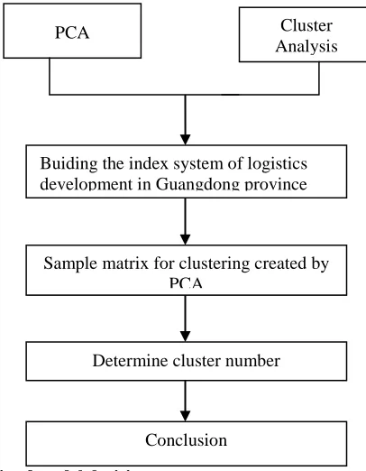
The following schematic indicates visually the method by which the developed operates.
Figure 1: Schematic of model decision process
PCA Cluster
Analysis
Buiding the index system of logistics development in Guangdong province
Sample matrix for clustering created by PCA
Determine cluster number
42
2.3.1. The city logistics development environment comprehensive evaluation PCA
model
2.3.1.1. General principle of the PCA (principal component analysis model)
PC Aaims to convert indicators into a handful of comprehensive index through dimension reduction. In statistics, principal component analysis is a simplified technology of data sets. It is a linear transformation. It transforms the data to a new coordinate system. It makes any data projection of the first big variance in the first coordinate (called the first principal component), the second big variance in the second coordinate (the second principal component) and so on. Principal component analysis often used to reduce dimension numbers, while keeping the data features which can contribution to the variance of a data set mostly. This is achieved by retaining low-order principal component, ignoring higher-order principal component. These low-order components always can retain almost all information of the data.
The basic principle of principal component analysis is using the ideas of dimension reduction; it is also a multivariate statistical method which converts the indicators into a handful of comprehensive index. Each of these indicators is relative, and information between each other will be overlapped to a certain extent. Therefore, principal component analysis can be used for the regional logistics development comprehensive evaluation in a province.
2.3.1.2. Steps of principal component analysis
Given n regions, p indicators, the original sample matrix will be
* ij n p
x* (x )
,
i
1, 2,...n; j 1, 2...p
First, we obtain standardized processing to eliminate the influence of different dimensions, which is
we define the standardized evaluation matrixX(X )ij n p , which is given as follows:
𝑋𝑖𝑗 =
𝑋𝑖𝑗∗ − ͞𝑋𝑖𝑗∗
𝑆𝑗∗
Where *
ij
X
is the samplemean of j-jth indicator, and Sj*is the samplestandarddeviation.
Calculating correlation coefficient matrix between indicatorsRp p , as well as its Eigen value
1 2... n 0
and eigenvectorej.
Now, we obtain the principal components as follows:
j j
Y Xe
The variance contribution rate of the jth principal component is
/
j j
a p, if the cumulative variance
contribution rate
1 q
j j
aa reaches the threshold (generally larger than 85%), using the top q
principal components
1, 2,... q
Y Y Y as comprehensive indicators which can best and comprehensively
explain the original p indicators.
Using the proportion of each principal component’s Eigen value of the total Eigen value as its weights of component comprehensive model.
1 1
( ), m 1, 2,..., q q
i i q
i m
m Y
F
43
Where F reflects the comprehensive strength of area logistics development, the higher value of F the better of region logistics development, the weaker conversely.
2.3.1.3. Cluster analysis model
Cluster analysis is a general terms that manipulate variables according to its features by multivariate analysis techniques. According to the different types of samples, these are divided into Q-type cluster analysis and R-type cluster analysis. Q-type cluster analysis refers to the sample clustering, while the R-type cluster analysis refers to the variable clustering, here we mainly used Q-type clustering. The purpose of cluster analysis is to divide objects into different classes according to certain rules. These classes are not given in advance, but determined in accordance with the data features. Sample observations in the same group are similar to each other to some degree; those in different groups have greater disparities.
2.3.1.4. Principle of cluster analysis
System clustering is a method of successive mergers; each specifies the distance between samples and between classes, letting n samples into a class of their own.
In the beginning, every sample is a class, the distance between classes and samples is the same; and then, merge two nearest classes; repeat, reduce a category at each time, successively looping until all samples classified in a class. However, it is meaningless that all samples are classified into a class, so that the process ceases when the class numbers reach a threshold. Hence, we obtain the result of clustering analysis. Nevertheless, it is surely a complex problem to determine the number of clusters, the clustering process can be visualized by binary hierarchical clustering diagram.
2.3.1.5. Steps of system clustering
Take a brief summary of system clustering; there are five parts as following: 1) Defining the distance among samples and the distance among classes; 2) Taking each Observation record as an individual category;
3) Calculating the distance between classes, and merge the nearest two classes, then the class number minus one;
4) If current class number greater than 1, turn back to step 3; 5) The end of the clustering.
2.3.1.6. The method of defining distance
We can know it is the key point for clustering that how to define the distance between samples and the distance between classes from the general steps of clustering. There are kinds of approaches for system clustering, but its implementation are basically the same. Euclidean distance was used in this study, the specific equation follows:
p
2 ij
1
d = ik jk
k
x x
Here, dijrepresents the distance between sample i and sample j, p is the number of samples.
The distance between the two classes is generally defined as the distance between some special
points in class. Here we have two classes GkandGL, in this study we used class average method to calculate the distance between classes, the specific formula is as follows:
KL 1 D
i k j L
ij x G x G K L
d n n
44
2.3.2. The construction of comprehensive evaluation index system for logistics
development
2.3.2.1. The principle of index selection
Comprehensive evaluation of logistics development is a complicated system engineering. In the process of the index selection, mainly follow the following principles:
a) Integrity, the selection of logistics development indicators should take the society macroeconomic environment, logistics infrastructure, logistics performance, human resource etc, into consideration.
b) Objectivity, index system should be objective and truly reflect the goals and the relationship between indexes, data must be objective and reliable.
c) Availability, each index should be univocal, easily accessible, and the calculation method should be concise.
d) Comparability, the selection of logistics development evaluation index system should be comparable across the region.
2.3.2.2. The comprehensive evaluation index system of logistics development
Based on the above principle, as well as the related literature and consult the opinions of the experts, we pick the following five aspects Indicators to establish a comprehensive evaluation index system of logistics development level, these indicators reflect the logistics development from different aspects.
a) Social and economic development, reflect the basis of social economy for logistics development. Including GDP(X1), per capita GDP(X2), disposable income(X3)
b) Transportation, including cargo throughput of port(X4), volume of freight traffic(X5), tonnage mileage(X6)
c) Human resource, including number of graduation from secondary vocational education(X7) d) Production, consumption of circulation, including gross farm production(X8), gross industrial
production(X9), Building gross(X10), total retail sales of consumer goods(X11), gross export(X12), gross import(X13)
e) Information development , including total of posts business(X14)
2.3.2.3.Research instance of logistics development evaluation in Guangdong province
Guangdong province earliest started logistics industry in China; logistics development evaluation plays an important role in logistics practice.
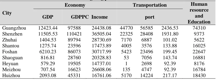
Therefore, the author selected the 2011 data of 21 cities in Guangdong province as the research objects, Specific data are shown in table 1:
Table 1: Evaluation index data of Guangdong province in 2011
City
Economy Transportation Human
resource and Education
GDP GDPPC Income port
Guangzhou 12423.44 97588 24438.08 44770 56585 2436.53 74310
Shenzhen 11505.53 110421 36505.04 22325 28408 1931.80 9373
Zhuhai 1404.53 89794 28730.69 7170 6887 101.02 5622
Shantou 1275.74 23596 17473.89 4005 3576 133.88 16025
Foshan 6210.23 86073 30717.99 5423 23496 199.45 22647
Shaoguan 816.81 28760 20328.83 53 7056 143.74 16881
Heyuan 579.29 19505 14737.01 1 2698 92.39 8176
Meizhou 707.54 16623 26608.06 135 4747 92.39 16784
45
Shanwei 550.55 18682 15751.37 564 1596 17.56 4226
Dongguan 4735.39 57470 39512.65 6848 10165 187.48 13943
Zhongshan 2193.2 70014 27699.71 5485 11439 94.28 7369
Jisangmen 1830.64 41062 23923.63 5914 8180 107.19 15666
Yanghiang 766.82 31491 16878.19 1121 2980 64.88 3875
Zhanjiang 1700.23 24163 17583.62 15539 8847 300.77 37320
Maiming 1745.31 29811 16113.39 2307 5202 118.35 40285
Zhaoqing 1324.41 33642 19039.65 2489 3342 45.36 22571
Qingyuan 1003.03 26957 17667.53 697 8038 136.96 12882
Chazhou 647.22 24169 15664.31 936 2970 130.88 4382
Jieyang 1225.86 20780 16878.89 1547 2280 34.08 7821
Yunfu 481.37 20302 16090.48 1206 2707 43.85 7955
Total Production
Technology development
City Agriculture Industrial Output
Contribution Output
Retail
Output Export Impact
Post telephone
service
Guangzhou 204.54 4140.59 436.38 5243.02 564.68 596.94 525.32
Shenzhen 6.55 4995.10 348.23 3520.87 2453.99 1685.76 404.40
Zhuhai 36.55 714.29 50.12 567.86 239.77 276.53 43.85
Shantou 73.76 592.86 56.84 972.21 59.53 28.35 60.13
Foshan 118.86 3735.29 135.66 1931.41 390.91 217.98 134.57
Shaoguan 113.16 298.26 48.97 383.99 7.22 10.57 21.68
Heuyan 72.39 285.90 20.65 188.04 19.16 8.77 19.36
Meizhou 143.99 227.52 55.14 372.79 10.94 2.71 35.69
Huizhon 116.51 1147.79 75.46 684.72 231.22 156.91 65.92
Shanwei 89.99 223.29 35.22 414.59 12.77 12.27 17.59
Dongguan 17.88 2288.41 77.79 1266.31 783.26 569.07 218.36
Zhongshan 58.45 1164.62 58.62 756.07 245.46 96.39 69.35
Jiangmen 138.36 953.21 44.05 759.15 122.52 54.37 50.34
Yangjiang 160.33 295.80 43.18 440.11 19.19 2.31 21.36
Zhanjiang 344.15 642.11 68.32 805.99 30.95 23.10 56.98
Maoming 319.24 645.80 50.86 842.86 5.99 3.25 39.23
Ziaoqing 226.40 535.42 51.87 389.71 33.08 24.04 32.28
Qingyuan 139.33 402.64 45.84 433.69 23.43 21.97 28.14
Chaozhou 45.97 333.27 19.66 287.73 27.09 14.72 21.70
Jieyang 128.70 687.87 47.09 573.45 37.92 7.32 35.57
Yunfu 119.72 181.35 23.11 167.58 8.84 5.05 16.18
According to principal component analysis model, standardized the above raw data (specific data are shown in table 3), disappear the dimensional effect.
46
Table 2: characteristic value and the variance contribution rate of each component
Elements Attributes Contribution Accumulated Contribution
1 2 3 4 5 6 7 8 9 10 11 12 13 14 10.331 2.290 0.552 0.414 0.154 0.153 0.044 0.032 0.018 0.006 0.003 0.002 0.001 0.000 73.790 16.355 3.945 2.955 1.100 1.092 0.317 0.229 0.130 0.040 0.023 0.014 0.010 0.001 73.790 90.145 94.090 97.044 98.144 99.236 99.553 99.782 99.913 99.952 99.975 99.989 99.999 100.000
From Table 2, we observe that the first principal components variance contribution rate is 73.79%,the first two Eigen values explain the variance of the total 90.145%, So the first two components has summed up the most of the information, the total variance contribution rate of the last 12 components is less than 10%. So this paper we will take two components as the main components which are Y1and Y2.Thus, this original 14 indicators convert into two new indicators, it plays the role of dimensionality reduction.
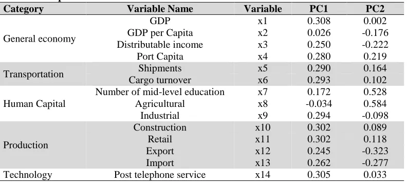
The calculation of feature matrix are shown in Table 3.
Table 3: Component matrix
Category Variable Name Variable PC1 PC2
General economy
GDP x1 0.308 0.002
GDP per Capita x2 0.026 -0.176
Distributable income x3 0.250 -0.222
Port Capita x4 0.280 0.219
Transportation Shipments x5 0.290 0.164
Cargo turnover x6 0.293 0.102
Human Capital
Number of mid-level education x7 0.172 0.528
Agricultural x8 -0.034 0.584
Industrial x9 0.294 -0.098
Production
Construction x10 0.302 0.089
Retail x11 0.302 0.118
Export x12 0.245 -0.323
Import x13 0.262 -0.277
Technology Post telephone service x14 0.305 0.033
According to the component matrix, we can get a linear combination of the first two principal components as follows:
Y1 = 0.306X1 + 0.265X2 + 0.250X3 + 0.280X4 + 0290X5 + 0.293X6 + 0173X7 – 0.035X8 +0.294X9 + 0.303X10 + 0.302X11 + 0.245X12 + 0.263X13 + 0.305X14
47
It can be seen that in a linear combination of the first principal component, in addition to the agricultural output X8, coefficient of the rest variables are nearly the same, only the variable X7 graduation number of secondary vocational is a little bit different. The first principal component explained 73.79% of the total information. It can be basically regarded as the comprehensive substituted indicator for GDP(X1), per capita GDP(X2), disposable income(X3), cargo throughput of port(X4), volume of freight traffic(X5), tonnage mileage(X6), number of graduation from secondary vocational education(X7), gross farm production(X8), gross industrial production(X9), Building gross(X10), total retail sales of consumer goods(X11), gross export(X12), gross import(X13), total of posts business(X14). It also reflects that the industries commercial economy and transportation as well as information technology have great impact on logistics. The second principal component mainly shows the influence on the demand of logistics service from agricultural development. Since the X13,X14 total import and export have higher negative load, we can conclude that the second principal component has impact on non-trading affairs.
The principal component integrated model as follows:
𝐹 = λ1
λ1+ λ2× Y1+
λ1
λ1+ λ2 × Y2
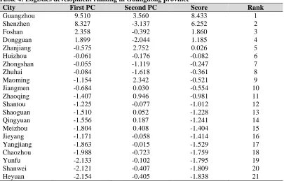
Here, F is comprehensive principal component values, represents logistics development, the larger of F the better of its logistics development. Meanwhile, the negative value doesn’t means the regional logistics development is poor, it just a relative value. Detailed in Table 4.
Table 4: Logistics development ranking in Guangdong province
City First PC Second PC Score Rank
Guangzhou 9.510 3.560 8.433 1
Shenzhen 8.327 -3.137 6.252 2
Foshan 2.358 -0.392 1.860 3
Dongguan 1.899 -2.044 1.185 4
Zhanjiang -0.575 2.752 0.026 5
Huizhou -0.061 -0.176 -0.082 6
Zhongshan -0.055 -1.119 -0.247 7
Zhuhai -0.084 -1.618 -0.361 8
Maoming -1.154 2.342 -0.521 9
Jiangmen -0.684 0.030 -0.554 10
Zhaoqing -1.407 0.946 -0.981 11
Shantou -1.225 -0.077 -1.012 12
Shaoguan -1.510 0.052 -1.228 13
Qingyuan -1.556 0.187 -1.241 14
Meizhou -1.804 0.408 -1.404 15
Jieyang -1.171 -0.058 -1.414 16
Yangjiang -1.863 -0.015 -1.529 17
Chaozhou -1.988 -0.723 -1.759 18
Yunfu -2.133 -0.102 -1.795 19
Shanwei -2.121 -0.407 -1.809 20
Heyuan -2.154 -0.405 -1.838 21
48
0.0 0.2 0.4 0.6 0.8 1.0 1.2 1.4 1.6 1.8 2.0 He Yuan
Shanwei
Yun Fu
Chao Zhou
Yang Jiang
Jie Yang
Qing Yuan
Shao Guar
Mei Zhou
Shan Tou
Zhao Qing
Jiang Men
Zhu Hai
Hui Zhou
Zhong Shan
Mao Ming
Zhan Jiang
Dong Guan
Fo Shan
Shen Zhen
Giung Zhou
have higher developed in foreign trade.Maoming, Shantou, Shaoguan and Zhaoqing, Qingyuan, Jieyang, Meizhou, Yangjiang, Chaozhou, Yunfu, Shanwei, Heyuan all are negative on the first principal component, it shows that all of them are needed to improve their economy. The second principal component of Zhanjiang, Maoming, Zhaoqing are greater than the others. This indicates that their agricultural development is better than others, but they need to improve theirforeign trading. Therefore, according to the scores for each city, the regional logistics development in Guangdong province is roughly divided into four levels.
The first level(Fi>2):Guangzhou, Shenzhen; the second level (1<Fi<2): Foshan, Dongguan; the third level (-0.6<Fi<1):Zhanjiang, Huizhou, Zhongshan, Zhuhai, Maoming, Jiangmen; the fourth level (Fi<-2): the rest of cities.
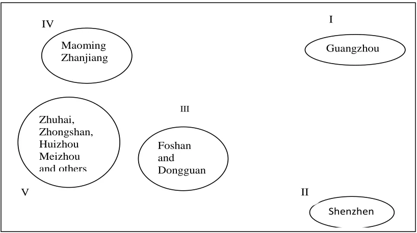
2.3.2.4. Logistics cluster in various cities in guangdong province
If analyzed in accordance with the general clustering methods, as many indicators calculated relatively tedious and error prone, prior to the analysis in view of the first two principal components obtained can reflect 90% of the original data information based on the main component, And these two components are not related to each other. So in front of the principal component analysis using two principal components indicator data obtained, consisting of cluster analysis of the sample matrix. According to average method for cluster analysis class level of logistics development in all regions of Guangdong Province, and draw the cluster diagram shown in Figure 1.
49 Maoming
Zhanjiang
Zhuhai, Zhongshan, Huizhou Meizhou and others
Foshan and Dongguan
Shenzhen
Guangzhou I
II III
V IV
2.3.2.5. Determining the number of the class
How to determine the numbers in each cluster is appropriate? This is a very difficult problem, which people have not found a satisfactory way yet to solve, but this is a problem that cannot be avoided. This study adopts the classification of the following several methods to determine the number of classes to achieve the comprehensive level of regional logistics development:
2.3.2.6. Threshold T
Via the observation of clustering in Figure 1, we gave thought to the appropriate threshold T, which requires the distance between classes should greater than T, so some samples may be unable to be classified. This method has strong subjectivity, which is its deficiencies. Observe the distance between classes T=1.4,two categories divided , respectively (1) Guangzhou, Shenzhen; (2)the remaining 19 cities; if T=1,three categories divided, respectively(1) Guangzhou;(2) Shenzhen ;(2)the remaining 19 cities; if T=0.7,four categories divided , respectively (1)Guangzhou;(2)Shenzhen; Dongguan; (3) Foshan; (4) the remaining 17cities;if T=0.5,it can be divided into five categories,respectively(1)Guangzhou;(2)Shenzhen;(3)Dongguan;(4)Foshan;Maoming;Zhanjiang;(5) the remaining cities.
2.3.2.7. The scatter diagram
If there is only two or three variables of the sample, we can determine the number of classes by observing the scatter diagram of data. Take the first principal components as the X axis, and the second principal components as the Y axis to draw the corresponding scatter diagram, as shown in Figure 2: Principal componentsby observation of the scatter diagram according to the scores of two principal components, the 21 cities of Guangdong Province can be divided into five categories:(1)
Figure 2: Cluster scatter
Guangzhou; (2) Shenzhen; (3) Dongguan; (4) Foshan; Zhanjiang; Maoming; (5) the remaining cities.
We denote the pseudo t2statistic as follows
:
𝑡
2=
DKL2
(WK+ WL) / (nK+ nL− 2)
𝐷𝐾𝐿2 = 𝑊𝑀− 𝑊𝐾− 𝑊𝐿 If is the incremental of the sum of squared residuals within the new
50
of the combined categories of GK and GL. The value of false t is expresses that the increment of the sum of squared residuals within the new category D2KL is greater than the sum of squared residuals within the GK and GL after GK and GL merged into GM. It shows that the two combined categories are separated, i.e. the effect of last clustering is much better. The pseudo t2statistic is a useful
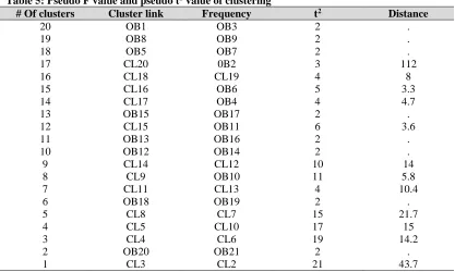
indicator to determine the number of categories, but it don’t have the distribution as random variables t2.In this study, the sample matrix consisting of two principal components uses SAS statistical software to cluster, and calculate the value of the false F and the value of the false t2, specific as follows in Table 5:
Table 5: Pseudo F value and pseudo t2 value of clustering
# Of clusters Cluster link Frequency t2 Distance
20 OB1 OB3 2 .
19 OB8 OB9 2 .
18 OB5 OB7 2 .
17 CL20 0B2 3 112
16 CL18 CL19 4 8
15 CL16 OB6 5 3.3
14 CL17 OB4 4 4.7
13 OB15 OB17 2 .
12 CL15 OB11 6 3.6
11 OB13 OB16 2 .
10 OB12 OB14 2 .
9 CL14 CL12 10 14
8 CL9 OB10 11 5.8
7 CL11 CL13 4 10.4
6 OB18 OB19 2 .
5 CL8 CL7 15 21.7
4 CL5 CL10 17 15
3 CL4 CL6 19 14.2
2 OB20 OB21 2 .
1 CL3 CL2 21 43.7
We observe from Table 5, the pseudo t2 value when divided into 1 class and 17 classes of pseudo t2
values were 112 and 43.7, although frequencies are greater. However, dividing into 1 class and 17 classes has no practical significance. When divided into 5 classes, the pseudot2value is 21.7.The greater the value of pseudo t2is reflected in a good clustering effect, therefore, dividing into4 classes is better. Based on the pseudo t2value the logistics development of 21cities in Guangdong province is
divided into 4 levels, respectively, these are (1) Guangzhou; (2)Shenzhen; (3) Dongguan, Foshan; (4) the remaining cities.
3. CONCLUSION
51
Table 6: Regional logistics development in Guang Dong province
Level Regions Cities
First level Guangzhou Shenzhen Guangzhou Shenzhen
Second level "two wings" area of Guangzhou Foshan, Dongguan
Third level East, west, north underdeveloped
area
Huizhou, Maoming, Zhanjiang, Zhuhai, Zhongshan, Jiangmen,
Shantou, Jyeing, Shanwei, Chaozhou, Yanjing, Qingyuan,
Zhaoqing,Shaoguan, Heyuan, Meizhou, Yunfu
Here we used principal component analysis and cluster analysis to evaluate the logistics development in Guangdong province. At the same time using threshold, scatter plot, pseudo t2
Statistic to determine the number of classes, here finally get the objective and convincing conclusion. It can provide important reference and basis for regional logistics planning.
From the result of principal component analysis, we can see that logistics development in Guangdong province is really imbalanced, except for Guangzhou, Shenzhen, Dongguan and Foshan. The remaining cities all need to enhance and improve their logistical construction activity. Maoming, Jiangmen, Zhuhai, Shanwei, Shantou should give greater importance to the advantages of the coastal cities. They should increase their construction of the logistical infrastructure and develop their logistical infrastructure better.
Views and opinions expressed in this study are the views and opinions of the authors, Asian Journal of Empirical Research shall not be responsible or answerable for any loss, damage or liability etc. caused in relation to/arising out of the use of the content.
References
Allen, J., Tanner, G., Browne, M., Anderson, S., Christodoulou, G., & Jones, P. (2003). Modeling policy measures and company initiatives for sustainable urban distribution. University of Westminster, London, United Kingdom.
Anderson, S., Allen, J., & Brown, M. (2005). Urban logistics-how can it meet policy makers’ sustainability objectives? J. Transp. Geography, 13, 71-81.
Betanzo-Quezada, E. (2012). A methodological study to integrated urban freight approach: The case of the metropolitan area of Queretaro, Mexico. An Regional Urban Studies [Digital]. Crainic, T. G, Ricciardi, N., & Storchi, G. (2004). Advanced freight transportation systems for
congested urban areas. Transp. Res. Part C, 12: 119-137.
Filippi, F., Nuzzolo, A., Comi, A., & Site, P. D. (2010). Ex-ante assessment of urban freight transport policies. Procedia-Soc. Behav. Sci., 2(3), 6332-6342.
May, A. D., Nelly, C., & Shepherd, S. (2006). The principles of integration in urban transport strategies. Transp. Policy, 13, 319-327.
May, A. D, Page, M., & Hull, A. (2008). Developing a set of decision-support tools for sustainable urban transport in the UK. Transp. Policy, 15, 328-340.
Patier, D., & Brown, M. (2010). A methodology for the evaluation of urban freight innovations. Procedia-Soc. Behav. Sci., 2(3), 6229-6241.
Ramanathan, R. (2001). A note on the use of the analytic hierarchy process for environmental impact assessment. J. Environmental. Management, 63, 27-35.