Article
SMALL ORDER PATTERNS IN BIG TIME SERIES:
A PRACTICAL GUIDE
Christoph Bandt
Institute of Mathematics, University of Greifswald, 17487 Greifswald, Germany; [email protected]
1 2 3 4
5 6 7 8
9
Abstract:Thestudyoforderpatternsofthreeequallyspacedvaluesxt, xt+d, xt+2dinatimeseries isapowerfultool.Thelag d ischangedinawiderangesothatdifferencesoffrequenciesoforder patternsbecomeautocorrelationfunctions.Similartoaspectrograminspeechanalysis,fourordinal autocorrelationfunctionsareusedtovisualizebigdataseries,asforinstanceheartandbrainactivity overmanyhours.Themethodappliestorealdatawithoutpreprocessing,outliersandmissingdata donotmatter. Onthetheoreticalside,westudypropertiesofordercorrelationfunctionsandshow thatthefourautocorrelationfunctionsareorthogonalinacertainsense.Ananalysisofvarianceofa modifiedpermutationentropycanbeperformedwithfourvariancecomponentsassociatedwiththe functions.
Keywords:permutationentropy;autocorrelation;timeseries;orderpattern
10
1. Order patterns fit big data
11
Few decades ago, when time series analysis was created, it did suffer from a lack of data. Now
12
the challenge is an oversupply of data. Old methods and models have to be modified, and new ones
13
have to be developed. Let us state the main requirements to new methods for big time series.
14
• Basic methods should be simple and transparent.
15
• Few assumptions should be made on the underlying process.
16
• Algorithms should be resilient with respect to outliers and artefacts.
17
• Computations should be very fast.
18
Classical probabilistic methods have problems with the second property. They often require
19
conditions like multivariate normal distribution which are not fulfilled in practice, or formulate their
20
conditions in terms of limits so that they cannot be checked. On the other hand, machine learning
21
procedures are in fashion, and very successful for specific purposes, but they do not have the first
22
property. They do not provide clear insight into the observed phenomena.
23
The analysis of order patterns in a signal fulfils all four requirements. It has been neglected until
24
recently when the tedious work of counting ‘larger’ and ‘smaller’ in a large series could be delegated
25
to a computer. Today, use of permutation entropy is well-established [1–3], and pattern frequencies
26
have been studied in particular for chaotic dynamical systems and heartbeat [4,5]. Here we continue
27
our efforts [6–8] to supply a theoretical foundation of ordinal time series analysis, concentrating on the
28
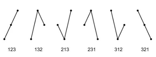
simplest patterns of length 3, depicted in Figure2below.
29
After years of doubt, we are now convinced that the study of order patterns in signals and
30
functions is interesting for its own sake, even from a theoretical point of view. It does not fit the
31
dominating analysis of smooth functions, and in [6] we found only few connections with the established
32
theory of stochastic processes. However, the emerging modern combinatorics of permutations [9–12]
33
will probably provide appropriate models.
34
This note will show that for many practical applications, order patterns are comparable or even
35
more appropriate than classical methods. Section 2 presents key concepts of the paper. In Section 3 we
36
explain the basic calculation of pattern frequencies, including treatment of ties and missing values.
37
Properties of order correlation functions are discussed in Section 5, leading to an analysis of variance
38
of permutation entropy. The main purpose of this paper, however, is a proof of concept by application
39
to biomedical signals, to speech and music, and to environmental and weather signals.
40
Figure 1.Respiration of a healthy volunteer during 24 hours of normal life. a: One minute of clean data. b: Mean flow for intervals of 30 seconds. c: Order correlation function ˜τ(d)for each minute.
Figure1gives a first example of a typical application. Data come from a cooperation with Achim
41
Beule (University of Münster and University of Greifswald, Department ENT, Head and Neck Surgery).
42
To study respiration in everyday life, two sensors measuring air flow intensity with sampling frequency
43
50 Hz were fitted to the nostrils of a healthy volunteer. This experimental setting was by no means
44
perfect. For example, mouth breathing could not be controlled. As a result, the data contain lots
45
of artefacts, and even the 3000 values of a ‘clean minute’ shown in Figure1a look pretty irregular.
46
Traditional analysis takes averages over 30 seconds to obtain a better signal, as shown in Figure1b.
47
Much more information is contained in a function ˜τ(d), defined below. Figure1c shows the collection
48
of these functions for all minutes of the signal, visualized like a spectrogram. We see phases of activity
49
and sleep, various interruptions of sleep, inaccurate measurements around 8 am, a little nap after
50
2 pm. Frequency of respiration can be read from the lower dark red stripe which marks half of the
51
wavelength. The upper light stripe marks the full wavelength: 4 s in sleep, 3 s or less in daily life.
52
2. Key concepts and viewpoints
53
We assume we have a time seriesx1,x2, ...,xT. To any three equally spaced valuesxt,xt+d,xt+2d
54
we can assign one of the six order patterns in Figure2. To the patternπ=123 we determine its relative
55
frequencypπ(d) =p123(d)in the time series, and this is done for each patternπ.. Details are described
56
in Section 3. Here we explain how to arrange and combine the six pattern frequencies. Patterns of
57
length 4 or longer are more difficult to understand and will not be studied in this paper.
Figure 2.The six order patterns of length 3
The important point is that we vary the lag or delayd- between 1 and 1000, say. Thuspπ(d)is
59
a function like the autocorrelation function. Both are obtained by a kind of averaging over a certain
60
time period. Our hope is thatsuch a function will express essential features of the process which generates
61
the data, and suppress unimportant individual properties of the observed series.Thuspπ(d)is considered as
62
an estimate of a probability which belongs to the underlying process. To justify this viewpoint, we
63
must make a stationarity assumption for the process: the probability of a pattern does not change
64
during time. This is a weak condition, for instance stationary increments in the usual sense will be
65
sufficient [6]. A stronger condition is already needed when we define an average valuexof thext. In
66
practice, stationarity is not fulfilled for a long series as in Figure 1. In such biomedical series it can
67
be assumed for small intervals of 1 minute, for which we determined thepπ(d). There may be a few
68
minutes where respiration drastically changes, but on the whole the stationarity assumption is natural
69
and appropriate.
70
It turns out that the pattern frequencies themselves are not so informative, but they can be combined to form better descriptions of the underlying process. Thepermutation entropyis
H(d) =−
∑
πpπ(d)logpπ(d), (1)
where the sum is taken over the six patterns in Figure2, or allm! permutations of some lengthsm.
71
In other words, we have the probability space of order patterns and take its Shannon entropy. The
72
permutation entropy is a measure of complexity of the underlying process [13] and has found lots
73
of applications: distinguishing chaotic and noisy dynamics, classifying sleep stages and detecting
74
epileptic activity from brain signals, etc.
75
A similar complexity measure introduced in [7,14] is thedistance to white noise
∆2(d) =
∑
π
pπ(d)− 1 m!
2
. (2)
White noise is a series of independent random numbers from a fixed distribution, and it is well known
76
that for this process, all pattern probabilitiespπ(d)are equal to 1/m! for lengthm, in particular 1/6
77
for length 3. We just take the quadratic Euclidean distance between the vectors of observed pattern
78
frequencies and the frequencies of white noise. There is an even simpler interpretation: the average
79
pattern frequency is always 1/m! , so thevariance of pattern frequenciesequals∆2/m! . In [8] it was
80
pointed out that ∆2can be considered as a rescaled Taylor approximation of H, and it has a more
81
convenient scale thanH.
82
Now let us come back to our six patterns of lengthm= 3. It turns out that four differences of pattern frequencies provide meaningful autocorrelation functions [6,7,14].
up-down balance β(d) =p123(d)−p321(d) =p12(d)−p21(d), (3)
persistence τ(d) =p123(d) +p321(d)− 1
rotational asymmetry γ(d) =p213(d) +p231(d)−p132(d)−p312(d), and (5) up-down scaling δ(d) =p132(d) +p213(d)−p231(d)−p312(d). (6) The names sound a bit clumsy, and the interpretation of the functions in Section 4 is not straightforward. However, it will be shown that these four functions include all information of the six pattern frequencies, that they are orthogonal in a certain sense, and form a variance decomposition of∆2given by the Pythagoras type formula
4∆2=3τ2+2β2+γ2+δ2. (7)
For the equal pattern probabilities of a white noise process all terms of this equation are zero. Thus the definitions were arranged so that white noise is a good null hypothesis for statistical tests. This aspect will not be worked out here. However, thevariance componentsof∆2are considered as some other ordinal autocorrelation functions and used in some applications, as Figure1c.
˜ τ= 3τ
2
4∆2 , β˜= β2
2∆2 , γ˜= γ2
4∆2 , δ˜= δ2
4∆2 . (8)
A stationary Gaussian process is completely determined by its mean, variance, and autocorrelation
83
functionρ(d), andτcan be directly calculated fromρ[6]. For stationary Gaussian processes, and more
84
general for all reversible processes,β,γ, andδare zero for everyd. Thus our correlation functions can
85
be considered as a tool for non-Gaussian and irreversible processes. Actually, calculation ofβ,γ, andδ
86
in our examples will show that processes in practice are mostly irreversible and non-Gaussian.
87
To conclude this introduction, let us explain what we call a ‘big time series’.. We assume thatwe
88
observe a continuous quantity in continuous time, like temperature, wind speed, blood pressure, intensity
89
of an electric or acoustic signal. Current sensor technology makes it possible to measure with big
90
accuracy as fast and as long as we want. On the one hand this means that valuesxtare rarely equal,
91
so cases of equality can be discarded. On the other hand, we have no smallest lagd. Althoughd=0
92
makes no sense, we can even think about taking the limitd→0. In practice, we must always discretize
93
the measurement, so we have a minimald=1. However, we could also measure with double speed
94
and thus work withd= 12.
95
The situation here is different from discrete dynamical systems, like logistic or Henon maps,
96
ARMA models, or RR-intervals of heartbeat where the state of the system changes step by step. All the
97
above concepts work well for those systems. However, such systems usually have a short memory so
98
that it suffices to consider a few small values ofd. Figure1c, wheredruns from 1 to 300, would not
99
show any structure. On the other hand, there are well-established methods for such systems. It also
100
makes sense to consider singlepπ(d), even for long patterns [2,4].
101
The challenge and bottleneck in time series analysis are the great continuous systems, where we
102
may observe interacting periodicities and dynamical effects over several scales. Below we mention
103
tides, with a daily, monthly and yearly scale, and biomedical signals with scales for heart, respiration,
104
slow biorhythms, day and night. Such kind of data must now be addressed.
105
3. Calculation of pattern frequencies
106
We consider a time seriesx1,x2, ...,xTwithTvalues. For a brain signal measured with 500 Hz for
107
8 hours,Tamounts to 15 millions. However, since we divide the series into smaller parts where the
108
underlying process is assumed to be stationary, the typical lengthTwill vary between 500 and 20000.
109
Any three consecutive valuesxt,xt+1,xt+2form one of the six order patterns, or permutations, shown
110
in Figure2. We also consider three valuesxt,xt+d,xt+2dwith a time lagd >1. The points represent
111
pattern 231, for instance, ifxt+2d<xt<xt+d. If there are tiesxs =xtor missing values, the pattern is
112
not defined. The initial time pointtruns from 1 toT−2d. The delay parameterdcan vary between 1
113
anddmax≤T/6, say, and has the same meaning as in classical autocorrelation. For fixedd, letnbe the
number of time pointstfor which a pattern is defined, andnπthe number of time points where we
115
have patternπ. Then the pattern frequency ispπ(d) =nπ/n.
116
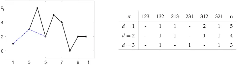
In Figure3we haveT= 10, and the valuex2is missing. Thust= 1 cannot be considered for
117
d =1, but for alld >1. Moreover, there are three equal valuesx5 =x9 =x10which excludet=8
118
ford =1, andt=5 ford=2. The resultingnπare listed in the table. We obtainp312(1) =2/5, for
119
instance.
120
π 123 132 213 231 312 321 n
d=1 - 1 1 - 2 1 5
d=2 - 1 1 - 1 1 4
d=3 - 1 - 1 - 1 3
Figure 3.Example time series and pattern frequenciesnπ. The dotted line indicatesd=2.
Since we have only six patterns, the statistics of pattern frequencies is excellent, even for short
121
time series likeT = 300. Form =6, for instance, we have 6! = 720 patterns and need a very long
122
time series to estimate all those pattern frequencies accurately. Permutation entropy would still work,
123
however, since it is an average over all patterns. Accuracy of estimates is one more reason to restrict
124
ourselves to patterns of length 3.
125
We can also determine frequencies of patterns 12 and 21 of length 2, forxt<xt+dandxt>xt+d.
126
Ford=1, we haven12 =n21=3, and ford=2 we getn12 =3,n21 =4. When we determineβ(d) =
127
p12(d)−p21(d), we obtainβ(1) =0,β(2) =−1/7. If we use the definitionβ(d) = p123(d)−p321(d)
128
in (3), we getβ(1) =−1/5,β(2) =−1/4. What is wrong?
129
There are several equations for thepπ= pπ(d)for fixedd. The basic equation is always accurate:
∑
π
pπ=1 for fixeddandm. (9)
The following equation is also accurate for probabilities in a stationary process [6].
p123+p132+p231=p12= p123+p213+p312. (10) To show equality on the left, divide the probability P(xt < xt+d) into three terms, depending on
130
whether xt+2dis above, between or below xtand xt+d. For the equality on the right, we consider
131
P(xt+d<xt+2d)and sum up three cases forxt.
132
Now if we calculate the frequencies for a time series withd = 1, then p12 is an average over
133
t=1, ...,T−1. To determinep12from the 3-patterns on the left, we average overt=1, ...,T−2. When
134
we take the 3-patterns on the right, we average overt= 2, ...,T−1. There is a marginal difference.
135
Moreover, the exclusion of missing and equal values can be different for patterns of different length, as
136
demonstrated above. Such marginal effects are the reason for the difference in the two expressions for
137
βin (3). Actually, (3) is a corollary of (10) andp321+p312+p213=p21, see [6]
138
Ford=1, such marginal effects are really harmless. For larged, however, they can become larger
139
since the margins of (10) will involvedtime points on the right and left end of the time series. This can
140
be a problem when we have a downward trend at the beginning of the series and an upward trend at
141
the end. For EEG brain data we helped ourselves defining the parts of the large series not by equal
142
length, but by zero crossings of the time series from the positive to the negative side [8]. Other data
143
may require other solutions for improved estimates of pattern frequencies.
Figure 4.Temperature inoCfor the first 10 days in January and July 1978, for 100 and 1000 days
Figure 5.Relative humidity in % for the first 10 days in January and July 1978, for 100 and 1000 days
4. First examples: weather data
145
To demonstrate the use of the above functions, we take hourly measurements of air temperature
146
and relative humidity from the author’s town: Greifswald, North Germany. The German weather
147
service DWD [15]. offers such data for hundreds of stations, where results are expected to be similar.
148
Measurements of our data started 1 January 1978. Figures4,5show temperature and humidity for the
149
first 10, 100, and 1000 days, and also for the first 10 days of July 1978. While in summer there is an
150
obvious day-night rhythm, this need not be so in winter when bright sunshine often comes together
151
with cold temperature. This effect is also visible in the bottom panel with data of almost three years.
152
We now look for correlation functions which describe the underlying weather process. We
153
calculate them bimonthly, and draw the curves for 35 years for the same season into one plot. When
154
they agree, we have a nice description of the underlying process - but this can never be perfect since
weather and calendar are not in one-to-one correspondence. Figure6compares classical autocorrelation
156
with our persistence function.
157
Figure 6.Autocorrelation and persistence for temperature (left part) and relative humidity (right part). The curves correspond to 35 consecutive years. The lagdruns from 1 to 49 hours. Each row describes a two-month period, from January/February up to November/December.
In winter (November to February) a day-night rhythm is not found, and all correlation functions
158
differ a lot over the years. From March until October, the day-night rhythm is well recognized, both
159
by autocorrelation and persistence, and both for temperature and humidity. Classical autocorrelation
160
curves coincide best at the full period maximum atd=24 hours while persistence accurately shows
161
the minimum at the half period of 12 hours. At the full period, there is a local minimum between two
162
maximum points, which will be explained in the next section. Both functions succeed in defining the
163
basic period within each window of 2 months (1461 hourly values). The coincidence over years seems
164
even better for persistence.
165
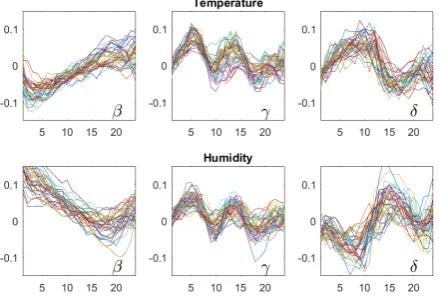
Figure 7. The functionsβ,γ, andδ, ford=1, ..., 24 hours, for July-August of 35 consecutive years. The upper row corresponds to temperature, the bottom row to relative humidity. Although there is considerable variation over the years, some common structure can be seen.
Is there more structure than day-night rhythm? Figure7shows the functionsβ,γ, andδfor
166
the summer season (July-August). In summer, the air warms up fast and cools down slowly which
167
explains whyβis negative for smalld. Humidity increases slowly and decreases fast, soβis positive
for smalld. In view of equation (11) below, theδfunctions also show opposite behavior. This was
169
found for all seasons. The structure ofγ, which is similar for temperature and humidity, was found
170
only in spring and summer (April to August), and we have no interpretation for it. Of course, the
171
functions will not improve weather prediction, but we think that any mathematical description of the
172
underlying process is of some value. For instance, the functions can be used to characterize or cluster
173
sites.
174
5. Properties of correlation functions
175
The classical autocorrelation functionρ(see [16,17]) measures the degree of coincidence of the
176
time series with a copy shifted bydtime steps. Thus autocorrelation is large for smalld. It will decrease,
177
and the rate of decrease reflects the memory of the underlying process. If we have a periodic dynamics,
178
autocorrelation will be large at the period, and small, mostly negative, at the half period. Moreover,
179
the sign ofρcan indicate an increasing or decreasing trend. The last point is not quite correct, because
180
a trend will exclude stationarity, and then, strictly speaking, we cannot estimate autocorrelation.
181
The direction of a trend is always indicated by β, and this can be consistent with the weak stationarity assumptions to estimate order pattern frequencies, for instance in the case of stationary increments with non-zero mean. The main purpose ofβ, as well as ofγandδ, is the description of certain asymmetries in the process. The up-down balanceβis positive for smalldif the process spends more time with increase than with decrease. When the process is stationary, this means that values will increase more slowly, and decrease faster. The functionsγandδare more difficult to interpret, but we can at least say thatδis tightly connected toβsince
δ(d) =β(2d)−β(d). (11) This follows from β(2d) = p123(d) +p132(d) +p213(d)−p321(d)−p312(d)−p231(d)and from the
182
definition ofβ. As in Section3, the equation holds for pattern probabilities of a process, and may have
183
a marginal error for frequencies of a concrete time series. This equation justifies the name up-down
184
scaling forδ.
185
Persistence is the most common and most important of our functions. It says how often a relation xt < xt+dorxt > xt+dwill persist in the next comparison ofxt+dwithxt+2d. Up to the sign, it can replace autocorrelation, and can be interpreted similarly. For smalld, persistence measures the degree of smoothness of the time series. When we have a smooth function, thenτ(d)tends to the maximal value 23 ford→0. We can also consider the complementary quantity
turning rate TR= p132(d) +p213(d) +p231(d) +p312(d) =2
3 −τ(d), (12)
which counts the frequencies of turning points (local maxima or minima) in the series. Obviously,TR
186
is a measure of roughness, or variation [18].
187
In this paper, however, the functions are chosen so that they are all zero for white noise - and for the slightly more general case of an exchangeable process where all patterns of Figure2have the same probability 16. In other words, white noise is the origin point of our coordinate system. This viewpoint is especially useful when we deal with noisy signals, for instance EEG brain data. All our functions are differences of pattern frequencies. Forτwe have
τ(d) = 1
3(2p123(d) +2p321(d)−p132(d)−p213(d)−p231(d)−p312(d)) . (13) Both (12) and (13) can be easily checked with (9). In the following, we systematically summarize
188
the properties of autocorrelation functions. For the sake of completeness, the next tables include
189
Spearman’s rank correlation, but not Kendall’sτ[19]. We think that for big time series, persistence
better reflects Kendall’s idea to measure correlation by order comparison. This is why we used the
191
letterτ.
192
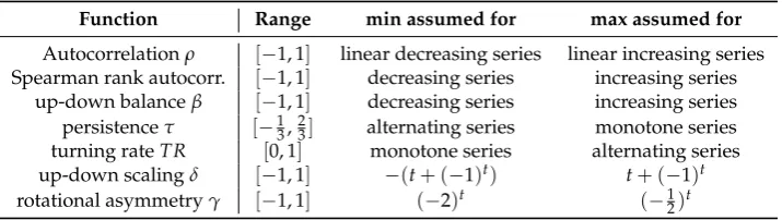
Table 1.Range and extreme cases for various correlation functions
Function Range min assumed for max assumed for
Autocorrelationρ [−1, 1] linear decreasing series linear increasing series Spearman rank autocorr. [−1, 1] decreasing series increasing series
up-down balanceβ [−1, 1] decreasing series increasing series persistenceτ [−13,23] alternating series monotone series turning rateTR [0, 1] monotone series alternating series up-down scalingδ [−1, 1] −(t+ (−1)t) t+ (−1)t
rotational asymmetryγ [−1, 1] (−2)t (−12)t
Table1shows the range of values for all correlation functions, adding for which series minimal
193
and maximal values are attained. An alternating series changes up and down at each step, like
194
xt= (−1)t+0.1·(uniform white noise)where the noise is added to avoid equal values. This works
195
ford=1, not for continuousd. Forγandδwe just gave an example series which may give a feeling
196
for what these functions measure.
197
Another viewpoint is symmetry. A function f(d)is even if f(−d) = f(d)and odd if f(−d) =
198
−f(d). For autocorrelation functions, even functions are those which assume the same values for a
199
time seriesx1,x2, ...,xTand its time-reversed seriesxT,xT−1, ...,x1. For odd functions, time reversal
200
will change the sign of the correlation function. We can also ask for invariance under change of sign
201
of the series, which gives−x1,−x2, ...,−xT, or for the combined change of sign and time reversal,
202
−xT,−xT−1, ...,−x1. The latter can be interpreted as a 180orotation of the graph of the series.
203
Table 2.Invariance of correlation functions under symmetries
Function Time reversal Negative function Rotation
ρ, Spearman,τ + − −
βandδ − − +
rotational asymmetryγ − + −
All autocorrelation behave well under these symmetries. They either remain invariant, in which
204
case we write a+in Table2, or they change sign in which case we note−. Persistence is an even
205
function likeρ, but our functionsβ,γ, andδare odd. This causes a discontinuity atd=0 unless the
206
value is zero there. Actually, none of our correlation functions is defined ford=0. We shall simplify
207
matters by restricting ourselves strictly positived. However, the problem will return when we consider
208
periodic series.
209
A time seriesx1, ...,xT is periodic with periodLifxt+L = xt fort = 1, ...,T−L. Theoretically,
210
none of our correlation functions is then defined ford = Lbecause there are only equal values to
211
compare. In reality, however, we have only approximate periodicity and can always determine values
212
ford = L. Nevertheless, some phenomena occur atd =L, 2L, 3L, ... and at half periodsd = L2,32L, ...
213
For a periodic time series, all autocorrelation functions are periodic with the same period - in practice
214
only approximately since only part of the generating mechanism works periodically. So it suffices to
215
considerd=Landd= L2.
216
For an even functionf(d)with periodLwe havef(d) = f(L−d)and hencef(L2+k) = f(L2−k).
217
That is, an even correlation function is mirror-symmetric with respect to the vertical lined=Las well
218
asd= L2. This is the case forρandτ. For an odd functiong(d)with periodLwe haveg(L−d) =−g(d)
219
and henceg(L2+k) =−g(L2 −k). In particularg(L2) =0. The graph ofgthen has a symmetry center
220
at(L, 0)and at(L2, 0). Both symmetry centers will be seen as zero crossings in the graphs ofβ,γ, andδ
even though theoretically we may have a discontinuity atL. For noisy series, the study of symmetries
222
of correlation functions can be quite helpful to recognize periodicities.
223
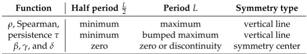
Table 3.Behavior of correlation functions of periodic series
Function Half period L2 PeriodL Symmetry type
ρ, Spearman, minimum maximum vertical line
persistenceτ minimum bumped maximum vertical line β,γ, andδ zero zero or discontinuity symmetry center
Let us now explain the behavior of persistence which we have already seen in Figure6. Ford= L2,
224
we always havext ≈xt+2din a series with approximate periodL. Thus ifxt+dis only a bit larger or
225
smaller, we cannot have pattern 123 or 321. This means thatτhas a clear minimum at L2. If the noise
226
level goes to zero, the value will approach the absolute minimum−13. This is the best way to determine
227
a period withτ.
228
Atd=Lthe behavior is more complicated, and different from the maximum ofρ. Assume that
229
much of the time series consists of monotone pieces, andxtis on an increasing branch. If we have the
230
exact periodL, and taked=L−εfor a smallε>0 thenxt>xt+d>xt+2dsince the shifted values are
231
further downwards on the repeating increasing branch. However, ford=L+εwith small positive
232
εwe havext < xt+d < xt+2dsince now the shifted values come further upwards on the repeating
233
branch. Only ford = Lwe theoretically havext = xt+d = xt+2dand can say nothing. In practice
234
there will be some noise which disturbs the monotone branches and changes our conclusion for small
235
ε. Anyway, left and right ofd = Lthe patterns 123 and 321 dominate and we have two maxima of
236
persistence there. But ford=Litself, the patterns 123 and 321 do not dominate anymore, and we get a
237
local minimum ofτ. This is what we call a bumped maximum. The height and width of the bump
238
decreases when the noise level goes to zero. See Figure6.
239
One can ask why among our four correlation functions, onlyτis even and the other three are odd. Actually we have six order patterns, so we could have three even and three odd functions. However, the patterns fulfil the sum condition (9) and another condition which directly follows from (10):
p132+p231−p213−p312=0 . (14)
Both of these conditions are expressed by even functions ofd, since the frequencies of a permutation
240
and its reversal, like 213 and 312, have the same sign in the equation. Thus we are left with four degrees
241
of freedom for our pattern frequencies, and it is natural to obtain three odd correlation functions.
242
The following theorem shows thatτ,β,γ, andδare an optimal choice of correlation functions
243
which explain in some way all the difference between our observed time series and white noise, a series
244
of independent random numbers. The information given by these functions is largely independent,
245
with the exception of dependence betweenβandδwhich cannot be avoided. This will be made precise
246
in a subsequent mathematical paper. Here we argue that certain vectors corresponding to the functions
247
are orthogonal, which can be the basis for ANOVA (analysis of variance) techniques.
248
Theorem 1(Pythagoras theorem for order patterns of length 3). For a process with stationary increments and an arbitrary lag d, the quadratic distance∆2 of pattern probabilities to white noise uniform pattern frequencies16defined in(2)has the following representation:
Proof. For arbitrary numbersq1,q2, ...,q6we have the following identity.
249
4 6
∑
k=1q2k = 2(q1+q6)2+2(q1−q6)2 +(q2+q3+q4+q5)2+ (q2−q3−q4+q5)2 +(q2+q3−q4−q5)2+ (q2−q3+q4−q5)2
If ∑qk = 0, the third square on the right is the same as the first. Now let q1 = p123−16,q2 =
250
p132−16,q3= p213−16,q4=p231−16,q5=p312−16, andq6=p321−16. Then∑qk=0 by (9), and the
251
last term on the right is zero by (14). According to the definitions of∆2,τ,β,γ, andδ, the identity turns
252
into the equation (15) of the theorem. This completes the theoretical part of the paper.
253
Figure 8.12 seconds of the song “Hey Jude” of The Beatles.a.The signal - mean of absolute amplitude over non-overlapping windows of 50 ms.b.The noisy places(x,d)for whichT∆2<15, drawn in
black. The vertical axis represents the lagd=1, ..., 30, considered as wavelength which ranges from 0 to 7 ms. Each column of the matrix corresponds to one windowx.
6. Case study: speech and music
254
One potential field of appplication of our correlation functions is speech and music: speech
255
recognition, speaker identification, emotional content of speech sounds etc. This field is dominated
256
by spectral techniques and by machine learning, and additional information on speech processes is
257
certainly welcome. We are not going into detail since we know this is hard work! Here we just analyze
258
the first 12 seconds of the song “Hey Jude” of The Beatles, to indicate what is possible.
259
The intensity of the signal is shown in Figure8. Since music is sampled with 44 kHz, there
260
are half a million amplitude values. For a rough analysis, we divide the large time series into 240
261
non-overlapping pieces, called windows, of length 50 ms. Thus there are 240 time series of length
262
T=2200 for which we can determine mean absolute amplitude and correlation functions. The delay
263
dwill run from 1= 1/44 ms tod =300 which is 7 ms. The functions will not be drawn as curves,
264
but as color-coded vertical sections of an image which describes the whole data set. The windows, or
265
columns of the matrix, are numberedx=1, ..., 240, the rowsd=1, ..., 300, written as 0..7 ms.
266
As a first experiment, we choose the points(x,d)for whichT∆2<15. They are colored black in
267
Figure8b. At these places we could perhaps still confuse the signal with white noise - according to
268
simulations in [8], the p-value is larger than 10−15. These places occupy 26% of the matrix, notably the
269
‘k’ of ‘take’ and‘s’ of ‘sad’ and ‘song’ with almost anyd. For all the other(x,d)Theorem 1 says that
270
some of our correlation functions are significant.
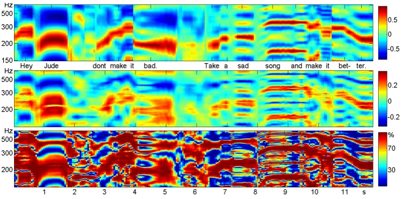
Figure 9.Correlogram (upper panel) and persistence (middle panel) of 12 s of “Hey Jude”. The scale ofdwas reverted and written as frequencies so that the melody can be read like musical notes. The bottom panel shows the percentage ˜τof∆2which is due to persistence.
Sliding window analysis of speech and music and visualization in a matrix is well-known from
272
the spectrogram where columns correspond to the Fourier spectrum of the windows. Since here, we
273
are satisfied with the melody - the so-called pitch frequency of the singer - we take the correlogram
274
instead, and compare with persistence in Figure9. For convenience, thed-scale is transformed into
275
frequencies - 500 Hz meansd=2 ms and 200 Hz meansd=5 ms. The maxima ofρand the bumped
276
maxima ofτare very clear for all voiced sounds. They describe the melody, and they do coincide.
277
The bottom panel of Figure9shows ˜τ= 3τ 2
4∆2, the percentage ofδ2which is due to persistence.
278
Clearly, persistence is the dominating function, with 80% of∆2at most places. But there also many
279
places with 30% and less where the functionsβ,γ,δform the larger part of∆2. Figure10shows some
280
phonemes which may be characterized this way.
281
Figure 11.Tides form an almost deterministic process with periodicities on the scale of days, months and years. Data from [20].
7. Case study: tides
282
Tides of the oceans are a well-studied phenomenon, and tidal physics is a science which has
283
developed over centuries. They form a good testbed for our correlation functions for two reasons. On
284
the one hand, there are excellent data series of water levels at many stations, provided for the USA
285
by the National Water Level Obersvation Network [20] over many years with 6 minute intervals and
286
few missing values. On the other hand, tides can be considered as an almost deterministic process
287
driven by the interaction of moon, sun, and earth, with geographical site and coastal topography of the
288
station as parameters. As Figure11shows, there are daily, monthly and yearly scales of periodicities:
289
tides at our selected places come two times a day, spring tides two times a month etc. Classical time
290
series will consider the data as a sum of sine waves, and there is an important theorem which says
291
that the ‘spectral measure’ for the frequencies of such a process is obtained as Fourier transform of the
292
autocorrelation function. From this point of view, our asymmetry functionsβ,γ, andδare negligible
293
and inappropriate. We shall show, however, that they do contain structural information on the process.
294
Figure 12.Water levels for three days in 2014, measured every six minutes at different stations in the USA. Data taken from [20], shifted and scaled for better visibility.
Since Anchorage, Alaska is situated at the end of a narrow bay, the tidal range (difference between
295
high tide and low tide) is 8 metres. In Los Angeles, California it is less than 2 m, and in Honolulu,
296
Hawaii, it is only half a metre. Order patterns cannot distinguish size of waves, we are only interested
297
in their structure! Moreover, it makes no sense to compare zero levels of stations, so they were shifted
298
for better visibility. For sake of completeness, Figure12includes Milwaukee at Lake Michigan where
299
there are no tides and differences are only 10 cm, caused by changes of wind and barometric pressure.
300
This series shows what fluctuations arise when data represent random weather change.
Figure 13. Correlation functionsβ, for one month in seven consecutive years, at the four places of Figure12. For a given month, each ocean station has its specificβ-profile.
The functionsβgiven in Figure13show that each of the ocran stations has its own profile which
302
did not change much in seven consecutive years. It did depend a bit on the season, however, so it was
303
taken for one month in each year. Since we have 240 values per day, we could afford even shorter
304
periods.
305
Experience shows that water comes fast and goes slowly, soβshould be negative for smalld.
306
This is clearly true for Milwaukee where no periodicity was found, and for Honolulu. For Anchorage
307
and Los Angeles, it is the other way round. For the three ocean stations,βhas a zero-crossing for
308
d≈12.5, and a ‘discontinuity’ atd=25. As explained in Section5, this corresponds to the basic daily
309
periodicity of 24.8 hours (the difference to 24 is caused by the moon).
310
Figure 14.Classical autocorrelation and order correlation functions for station Anchorage in January. Persistence reflects the diurnal rhythm. The asymmetry functionsβ,γ,δall show a very specific structure which remains stable through seven consecutive years. In contrast,ρdoes not seem to contain much structural information.
Figure 14 shows all order correlations for Anchorage for the month January. Both the
311
autocorrelation and persistence express the fact that there are two periodicities with periods of 12.5
312
and 25 hours. Forρ, the maximum at 25 is larger than the first maximum at 12.5 while the minimum at
313
19 is not smaller than the first minimum at 6. For persistence, the maximum at 25 has a small bump
314
while the maximum at 12.5 has a very large bump since it is a also a minimum corresponding to 25.
The functionsβ,γ,δall show a sharp structure which is preserved thorough consecutive years. This is
316
no proof that they contain more information thanρbut it is an argument for further study of these
317
functions.
318
Figure 15. The division of∆2into components described in Theorem 1, illustrated for the tides at Anchorage in the years 2013 and 2014 in sliding window analysis. From top to bottom, the four panels correspond to the function ˜τwhich takes the largest part of∆2, to ˜β, ˜γand ˜δ.
Finally we check Theorem 1 with the tides data of Anchorage in Figure15. Windows of length
319
1242 (5 days and 4.2 hours - just 5 main periods) were used for the years 2013 and 2014. For good
320
resolution, the step size is half a day, so successive windows overlap by 9/10 of their length. The lagd
321
was restricted to the time between 10.5 and 14.5 hours, around the first the important period 12.5 hours
322
where∆2is large. Roughly speaking, the picture shows how the position and width of the main bump
323
ofτin Figure14changes with time. There are small waves which describe the bimonthly period, and
324
long waves describing biyearly periodicity.
325
It can be seen how the different components fit together, with ˜τas dominant component. The
326
average value of ˜τwas 76% , followed by 15% for ˜β, 6% for ˜δ, and 2% for ˜γ. Since Theorem 1 holds
327
for probabilities of the process and here we have frequencies from data, there is a marginal error,
328
as explained in Section3. Sincedis between 105 and 145, this error could be rather large. Here the
329
average error is 0.5% . There are very few places(x,d)where the error is more than 1% , the maximum
330
was 2% .
331
This example shows that the order correlation functions ˜τ, ˜β, ˜γand ˜δcan also detect structure in
332
data, even though they are squares and lack the information of the sign of the original functions. In
333
the present case, as well as in Figure1c these relative quantities are more informative than the original
334
ones.
335
8. Case study: particulates
336
In the previous section, we had an almost deterministic process with excellent data. Now we
337
consider the opposite situation: measurements of particulates PM10 (aerodynamic diameter smaller
338
than 10µm). Such data, measured by a kind of vacuum cleaner with a light sensor for the dust, are
339
notoriously noisy. Dust will not come uniformly, it will rather form clusters of various size. Although
340
measurements can be taken several times in a second, they are averaged automatically at least over
341
several minutes. In Figure16we consider hourly values from the public database [21] for the station
3215 at Trona-Athol in San Bernardino, California. They were transformed to logarithmic scale to
343
reduce the influence of large values. Such a transform does not change order patterns.
344
Figure 16.Particulate measurements are notoriously noisy. They show a weak daily and yearly rhythm which can hardly be detected from the data. The PM10 measurements for station 3215 Trona -Athol at San Bernardino, California are from the public database [21].
There are 13% of missing values, some of which can be detected in the upper panel of Figure
345
16. They affect the estimation of autocorrelation much more than estimation of order correlation
346
functions. This can be seen in Figure17where all functions where determined for 12 successive years.
347
The variation is of course a bit larger than in the corresponding Figure14for the tides. The values
348
of the order correlations are about three times smaller than those for the tides. The important point,
349
however, is the consistent structure of the order correlation functions. It is much better than classical
350
autocorrelation or∆2in the upper row. Persistence shows a loss of intensity from one up to six days,
351
though not as strong as autocorrelation. However, the structure ofβ,δ, and evenγremains almost
352
unchanged from day 1 to day 6.
353
Figure 17. Correlation functions for hourly particulate measurements at San Bernardino [21] in 2000-2011. Each of the 12 curves corresponds to one year, in order to check consistency of correlation structure over the years. The functionsβ,δ, andγshow similar structure from day 1 to day 6.
To perform a sliding windows analysis with these data, we take windows of length 1200, that
354
is 50 days. Smaller windows do not provide sufficiently accurate estimates. Probably the situation
355
would be better if the data were measured every 6 minutes like tides above, even though there were
larger variations. Figure18shows that the daily rhythm appears mainly in summer, not in winter,
357
similar to temperature in Section4. Thus the curves of Figure??are obtained mainly from the summer
358
measurements. The strength of daily rhythm and the ‘length of summer season’ varies over the years.
359
Figure 18. Sliding window analysis ofapersistenceτ(d) andbup-down balanceβ(d)for hourly particulate measurements at San Bernardino 1997-2011 [21]. The lagdruns from 1 to 72, that is 3 days, on the vertical axis. Overlapping windows of 50 days were used. Daily rhythm is present mainly in summer, in bothτandβ.
9. Case study: brain and heart signals
360
The examples in Sections4,7, and8were presented as proof of concept, with the idea to encourage
361
readers to work out the applications in a more careful way. For biomedical data, however, the author
362
has done a careful study [8,14,18] of data published by Terzano et al [22] at physionet [23] which seems
363
very promising. Three types of data were considered, as indicated in Figure19: the noisy EEG brain
364
data (electroencephalogram), the well-known heart ECG (electrodardiogram), and the rather smooth
365
plethysmogram which measures the blood flow at the fingertip.
366
Figure 19. Biomedical signals: 8 seconds of a electroencephalogram, an electrocardiogram and a plethysmogram. Order correlation functions seem to apply to all of them.
In [8] it was found that the function∆2can distinguish sleep stages from the EEG data without
367
any further processing. In [18] it was noted that it is actually the persistence, or turning rate, the main
368
component of∆2, which can be taken as measure of sleep depth. For all healthy control persons and
369
a number of patients with different sleep problems, the results are as impressive as Figure20where
370
manual annotation by a medical expert and turning rate are almost parallel. The definition of sleep
371
depth is a complicated and controversial issue among physicians, and a pure mathematical definition,
372
even if it is not perfect, could be helpful.
Figure 20.Coincidence of sleep stage annotation by a medical expert and turning rate ford=8 ms of two EEG channels [18]. Original data from Terzano et al. [22].
So far, the author could not reproduce this result with more recent data. Actually, there are huge
374
databases of sleep data in different countries. But these data are not of the same quality as those of
375
[22] for two reasons. On the one hand, since there are so many data, they are sampled not at 500 Hz
376
but only at 200 Hz or less. On the other hand, EEG data are contaminated by the field of the electrical
377
power net with 50-60 Hz frequency. It is quite an effort to avoid this influence, especially in a hospital
378
environment. Since conventional evaluation of EEG data considers wavelength of at least 50 ms,
379
experts are content with this type of data. The standard preprocessing is a low-pass filtering with a
380
cutoff of 40 Hz, say. For determining the persistence or turning rate atd≤8 ms, or frequency≥130 Hz,
381
however, the 50 Hz noise of the power net is a real obstacle. This also holds for the ECG.
382
Figure 21.Theorem 1 for the plethysmogram over a whole night. From top to bottom: ˜τ, ˜β, ˜γ, ˜δ. The bottom panel contains the error of the equation of Theorem 1 on a scale from 0 up to 1% . Data of person n3 from Terzano et al. [22].
The plethysmogram is determined by a light sensor, and can be measured without power noise
383
contamination. Nevertheless, it is mostly measured at low frequencies like 30 Hz, because of its smooth
384
appearance. Perhaps there is also a fine structure for higher resolution which can be studied by order
methods. We conclude this paper with a Figure21 which shows the validity of Theorem 1 for a
386
plethysmogram of [22].
387
Acknowledgments:The author thanks Bernd Pompe for discussions over many years, and for his opinion on
388
the unpublished paper [14] on which part of this work is based. Costs to publish in open access were covered by
389
Deutsche Forschungsgemeinschaft, project Ba1332/11-1.
390
Conflicts of Interest:The author declares no conflict of interest.
391
Bibliography
392
1. Amigo, J.; Keller, K.; Kurths, J. Recent progress in symbolic dynamics and permutation complexity. Ten
393
years of permutation entropy. Eur. Phys. J. Special Topics2013,222, 247–257.
394
2. Amigo, J.M.Permutation complexity in dynamical systems; Springer Seires in Synergetics, Springer: Berlin,
395
2010.
396
3. Zanin, M.; Zunino, L.; Rosso, O.; Papo, D. Permutation entropy and its main biomedical and econophysics
397
applications: a review. Entropy2012,14, 1553–1577.
398
4. Parlitz, U.; Berg, S.; Luther, S.; Schirdewan, A.; Kurths, J.; Wessel, N. Classifying cardiac biosignals using
399
ordinal pattern statistics and symbolic dynamics. Computers in biology and medicine2012,42, 319–327.
400
5. McCullough, M.; Small, M.; Iu, H.; Stemler, T. Multiscale ordinal network analysis of human cardiac
401
dynamics. Philosophical Transactions of the Royal Society A: Mathematical, Physical and Engineering Sciences
402
2017,375, 20160292.
403
6. Bandt, C.; Shiha, F. Order patterns in time series. J. Time Series Analysis2007,28, 646–665.
404
7. Bandt, C. Permutation Entropy and Order Patterns in Long Time Series. InTime Series Analysis and
405
Forecasting; Rojas, I.; Pomares, H., Eds.; Contributions to Statistics, Springer, 2015.
406
8. Bandt, C. A new kind of permutation entropy used to classify sleep stages from invisible EEG
407
microstructure. Entropy2017,19, 197.
408
9. Bóna, M.Combinatorics of permutations; Chapman & Hall/ CRC, 2004.
409
10. Elizalde, S. A survey of consecutive patterns in permutations. arXiv150411.07265.
410
11. Elizalde, S.; Noy, M. Consecutive patterns in permutations.Adv. Appl. Math.2003,30, 110–123.
411
12. Glebov, R.; C., C.H.; Klimosova, T.; Kohayakawa, Y.; Král, D.; Liu, H. Densities in large permutations and
412
parameter testing. arXiv1412.5622v3.
413
13. Bandt, C.; Pompe, B. Permutation entropy: a natural complexity measure for time series. Phys. Rev. Lett.
414
2001,88, 174102.
415
14. Bandt, C. Autocorrelation type functions for big and dirty data series. arXiv1411.3904.
416
15. DeutscherWetterdienst. Climate Data Center. ftp://ftp-cdc.dwd.de/pub/CDC/observations_germany.
417
16. Brockwell, P.; Davies, R.Time Series, Theory and Methods, 2 ed.; Springer: New York, 1991.
418
17. Shumway, R.; Stoffer, D.Time Series Analysis and Its Applications, 2 ed.; Springer: New York, 2006.
419
18. Bandt, C. Crude EEG parameter provides sleep medicine with well-defined continuous hypnograms.
420
arXiv1710.00559.
421
19. Ferguson, S.; Genest, C.; Hallin, M. Kendall’s tau for serial dependence. Canadian J. Stat.2000,28, 587–604.
422
20. NationalOceanicandAtmosphericAdministration. National Water Level Obersvation Network. https:
423
//www.tidesandcurrents.noaa.gov/nwlon.html.
424
21. California. Air Resources Board. www.arb.ca.gov/adam.
425
22. Terzano, M.; Parrino, L.; Sherieri, A.; Chervin, R.; Chokroverty, S.; Guilleminault, C.; Hirshkowitz, M.;
426
Mahowald, M.; Moldofsky, H.; Rosa, A.; Thomas, R.; Walters, A. Atlas, rules, and recording techniques for
427
the scoring of cyclic alternating pattern (CAP) in human sleep.Sleep Med.2001,2, 537–553.
428
23. Goldberger, A.; Amaral, L.; Glass, L.; Hausdorff, J.; Ivanov, P.; Mark, R.; Mietus, J.; Moody, G.; Peng, C.K.;
429
Stanley, H. PhysioBank, PhysioToolkit, and PhysioNet: Components of a New Research Resource for
430
Complex Physiologic Signals. Circulation2000,101, e215–e220. database atwww.physionet.org.