1
MASTER THESIS
The Modularity of the Resource
Utilization Model in Python
Dennis Windhouwer
Department of Computer Science
University of Twente
Supervisors
prof.dr.ir. Mehmet Aksit
dr. Pim van den Broek
dr.ing. Christoph Bockisch
ir. Steven te Brinke
1
1. Introduction 1
1.1 Goals and Motivation ... 1
1.2 Approach ... 2
2. Resource Utilization Model 3
2.1 RUMs ... 3
2.2 Requirements of RUM Library ... 4
3. RUM Library 6
3.1 Functional Component RUMs ... 6
3.1.1 Service Invocation Interception... 6
3.1.2 State Machine ... 8
3.2 Optimizer Component RUMs ... 11
3.2.1 Optimizer Interjection ... 11
3.2.2 Query Capabilities ... 14
4. Example programs 19
4.1 General Structure ... 19
4.1.1 The world ... 19
4.1.2 The vehicle ... 19
4.1.3 Controller ... 20
4.2 Object-Oriented Program ... 20
4.3 RUM style Program ... 21
5. Modularity Metrics 24
5.1 Complexity ... 24
5.2 Cohesion ... 25
5.3 Coupling ... 28
6. Results 30
6.1 Measurements ... 30
6.1.1 Object Oriented program ... 30
6.1.2 RUM style program ... 32
6.2 Discussion ... 36
6.2.1 Other languages ... 37
7. Possible Improvements 41
Bibliography 45
also be interjected between any two components seamlessly, and the optimizers can determine how they can trigger desired state transitions in order to change the state of a RUM to a state with a more desired resource behavior.
In order to investigate the modularity of the RUM style, we first implemented an example program in the object-oriented style, using design patterns [11]. A functionally similar program was then also implemented in the RUM style, using the created library. These programs were then compared on their modularity.
1.2
Approach
To determine the modularity of the Resource Utilization Model in Python, we compared a program implemented in the RUM style, to a functionally similar program implemented in the object-oriented style with design patterns [11].
First we investigated how to measure the modularity of the resource utilization model. We identified several traits which we wanted to measure, and then investigated suitable metrics for measuring these traits.
Next, we implemented a program in the object-oriented style. This was a best effort at creating a modular object oriented program. By first creating this program, and ensuring it was as a modular as possible, influences from the RUM style on the program’s design could be minimized.
Then we created the development environment, as the program in the RUM style cannot be
implemented without it. The development environment was designed to be highly extensible, so that new functionally can easily be added to it, and so existing functionality can be extended.
Once the development environment was completed, we created a program in the RUM style, functionally similar to the earlier created object-oriented program. Work on this program continued until it too, was as modular as possible.
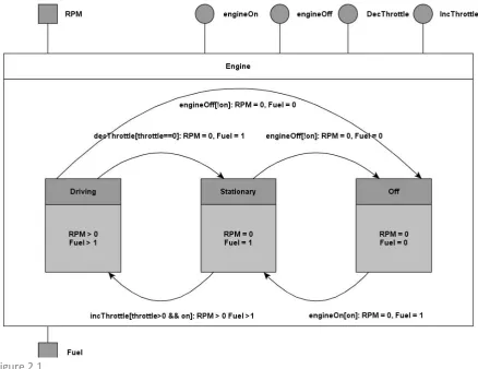
Figure 2.1
A user component can use the provided services in order to manipulate the engine. An optimizer component can then be interjected between the user component and the engine in order to manipulate the resource consumption and production of the engine. The following is an example of such an optimization. When the car has to stop in front of a railroad crossing, the optimizer can use information about average wait times at this crossing to determine whether the engine should remain in stationary mode, or whether it would be better for the fuel consumption to turn the engine off, and then back on once the crossing is clear. If it determines that it is better to keep the engine in stationary while the user is attempting to turn it off, then the optimizer would keep the engine running.
2.2
Requirements of RUM Library
The description of the RUMs and their workings shows several requirements which the RUM library will need to fulfill. As mentioned, service invocations can trigger state transitions, changing the state a RUM is in. But, as discussed in chapter one, one of the aims of the RUM method is to separate the functional concerns from the optimization concerns. If a component has to inform a RUM by calling a RUM’s method every time a service invocation occurs, then this will couple the component to the RUM. This would prevent the separation of the functional concerns from the optimization concerns. Thus the RUM needs to be capable of intercepting relevant service invocations without help from the component to which the service belongs.
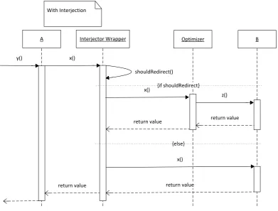
should instead be interjected between the components without the components code reflecting this. Calls from the user component to the functional component should then automatically be redirected to the optimizer without either component being aware of it.
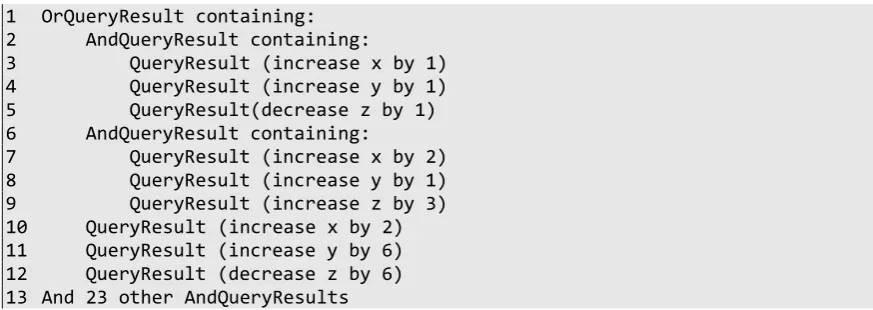
When an optimizer wants to modify the resource behavior of a component by changing the state of its RUM to a more desired state, then the optimizer needs to be capable of finding out which service invocations it must invoke, and in which order, so it can cause a transition to this more desired state. Information about these state transitions is contained in the RUM’s state transition diagram. The states, and state transitions, thus need to be declared and stored in such a way that an optimizer can introspect them, allowing the optimizer to determine which services need to be invoked.
From these requirements, we conclude that the development environment should:
- Allow RUMs to intercept service invocations.
- Provide a way to declare introspectable states and state transitions for a RUM. - Allow for the interjection of optimizer components between functional and user
components.
of state transitions which need to be checked by the RUMs which were interested in the invoked service, and on the amount of operators which these transitions contain. In the case of a single RUM, with a single state transition per state, each with a single operator, the performance impact was found to be around 8 microseconds.
A B
B.x() A.y()
return value No Interception
A Interceptor Wrapper
B.x() A.y()
return value With Interception
B
B.x()
return value
RUMs
CheckForStateTransition
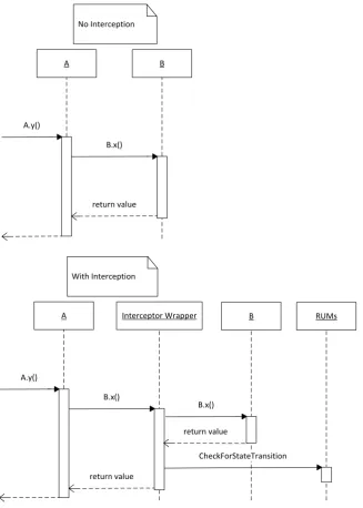
Figure 3.1.1.1 Interceptor wrapper sequence diagram
Another wrapper has also been implemented. When this wrapper is invoked, it first creates a dictionary containing the names and values of all the variables of the component to which the wrapped method belongs. Then it invokes the wrapped method. Once the wrapped method has returned, the wrapper again creates a dictionary containing the names and values of all the variables of the component. These two dictionaries thus contain all the values from before and from after the execution of the intercepted service. The wrapper then informs the Interceptor module about which service was invoked, and supplies the Interceptor module with these two dictionaries. The
Interceptor module passes these two dictionaries on to the RUMs. These two dictionaries are passed on all the way down to the operands and operators of a state transition, allowing for the
Figure 3.1.2.1 State diagram
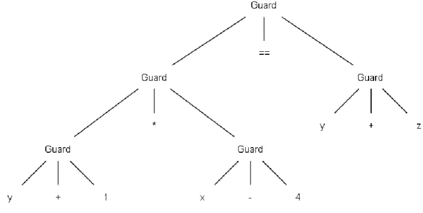
In order for the optimizer to determine how it can cause a state transition, the guard part of the transition also needs to be introspectable. An earlier investigation into suitable programming mechanisms [18] showed that using classes to build an AST tree, is an introspectable and very extendable solution for defining the guard part of state transitions. Figure 3.1.2.2 shows an example of such an AST tree. This AST tree represents the following expression: (y+1)*(x-4)==(y+z). It contains a total of five binary operators. In the tree each operator, together with its two operands, is
contained inside a Guard class. In this figure, the values of x, y and z represent
FieldVariableOperands. The +, -, * and == signs represent Operator classes. Both the Guards, FieldVariableOperands and Operator classes are explained below.
Figure 3.1.2.2 State transition
4.3
RUM style Program
The RUM style program has moved the resource behavior of the propulsion, gearbox and vehicle out of their classes and into the PropulsionRUM, gearboxRUM and vehicleRUM classes. Instead of the strategy pattern, it has two optimizer classes and one OptimizerRUM.
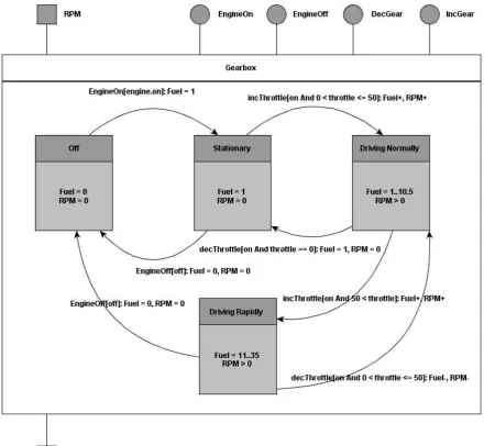
Figure 4.3.1 PropulsionRUM
This RUM intercepts four service invocations from the propulsion. These are the services responsible for turning the engine on and off, and the services responsible for increasing and decreasing the amount of throttle used by the propulsion. These services can cause transitions between the states as noted in figure 4.3.1. While figure 4.3.1 does not show it to keep the image clear, there is also a possible transition from the ‘Driving Normally’ state to the ‘Off’ state, similarly to the other transitions to the ‘Off’ state from the other states.
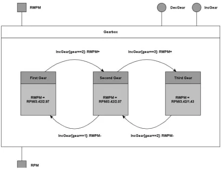
Figure 4.3.2 GearboxRUM
The GearboxRUM is responsible for managing the resource behavior of the gearbox. As shown in figure 4.3.2, it contains one state for each gear, each state having a different ratio. The actual gearboxes in the RUM and O-O programs have six gears, not three, but in order to keep the example clear we only show three in this figure. The resource which the gearbox consumes is RPM and the resource which it produces is rotations of the wheel per minute (RWPM). Each state has its own ratio, equal to the ratios of the gears in the Object Oriented program. The states all share the same differential ratio. In figure 4.3.2, this differential ratio is 3.42, while the first gear’s own ratio is 2.97. This RUM intercepts two service invocations from the gearbox. These are the service responsible for increasing the gear, and the service responsible for decreasing the gear.
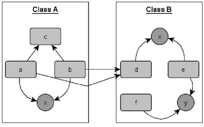
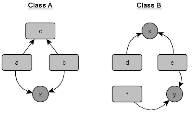
getters and setters, thus many methods end up using these getters and setters instead of accessing the instance variables directly. In LCOM, these methods are treated as dissimilar. There are also many cases where methods exist which do not directly access instance variables, but are coded entirely in terms of other methods of their class, which then do access these instance variables. In order to satisfy LCOM, these methods could certainly be merged into one big method, but all this achieves is to increase code duplication and the complexity of the methods in question. Figure 5.2.1 contains an example in class A, where improving cohesion would also increase code duplication. Method c uses no instance variables, but is called by both methods a and b. removing method c and moving its functionality into methods a and b would improve LCOM, while also adding undesired code duplication and complexity. So clearly this is not desired, and LCOM falls short when it is used to measure classes with such methods.
figure 5.2.1
A newer version of LCOM by Martin Hitz and Behzad Montazeri [12] addresses these issues. Their version of LCOM considers methods A and B to be cohesive if they access the same instance variable, or if A calls B, or if B calls A. After determining the related methods, a graph is drawn, connecting all related methods to each other. LCOM then equals the number of connected groups of methods in this graph. A value of 1 represents a cohesive class, where all methods are connected either directly or indirectly, while a value greater than 1 represents a class which can be split up into multiple smaller classes. Figure 5.2.2 shows the LCOM graphs for both classes from figure 5.2.1. Each graph contains one fully connected group, so both classes have an LCOM value of 1. While this version of LCOM shows into how many classes a measured class can be refactored, the value given by LCOM does not give any information about the size of the respective graphs. If two classes, C and D, both have an LCOM value of two and each have ten methods, with class C having two graphs with nine and one methods respectively, and class D having two graphs with five methods respectively, then clearly class C is much more cohesive than class D, but the metric does not show this. This is where our other chosen metrics, Tight Class Cohesion and Loose Class Cohesion, come in.
before leaving the class. Methods are considered indirectly connected if methods are not directly connected, but are connected through other methods, for example in figure 5.2.1, method d is connected to e and e is connected to f, thus d and f are indirectly connected through e.
figure 5.2.2
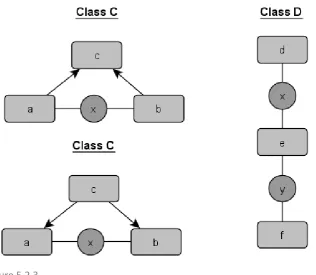
The value of TCC is then computed by dividing the amount of connections by the maximum number of possible connections (NP), which is N*(N-1)/2, where N is the number of visible methods. The value of LCC is computed by adding the amount of direct connections to the amount of indirect connections, and then dividing this sum by the maximum number of possible connections. LCC is thus always greater than or equal to TCC. Figure 5.2.3 shows the connections between the methods for TCC and LCC, using the two classes from figure 5.2.1. Assuming that all methods are public, then both classes A and B have three public methods, so the maximum number of possible connections is three for each class.
Direct connections in figure 5.2.3 are represented by a straight line between two methods, with a circle interrupting the line, containing the name of an instance variable which both of the methods use. A direct connection can thus be seen between methods a and b, d and e, and methods e and f. Class A thus has one direct connection, class B has two direct connections. As can be seen, we have also added a class C, this class is similar to A, except that method c now calls methods a and b, instead of a and b calling c. The amount of direct connections in class C is three, as the call tree starting from method c includes both methods a and b, and thus includes access to instance variable x. Thus the TCC values for classes A, B and C are respectively: 1/3, 2/3 and 1. As for the indirect connections, class A does not contain any as the call tree from method c never comes in touch with any other methods. Class B does contain an indirect connection, methods d and f are indirectly connected through method e. Class C does not contain any indirect connections as all connections are direct. Thus the LCC values for classes A, B and C are respectively: 1/3, 1 and 1.
method is visible or not greatly affects the scores produced by TCC and LCC. Class B scored 2/3 for TCC and 1 for LCC, which means it’s quite cohesive. Class C scored 1 on TCC and 1 on LCC, meaning it is maximally cohesive.
figure 5.2.3
As can be seen, one of the main differences between TCC/LCC and our chosen version of LCOM is seen when a class has a public method which does not access any instance variables, but is accessed by another method. LCOM considers these methods to be cohesive, but TCC and LCC do not. Both metrics thus have their advantages and disadvantages, LCOM shows how many different groups of connected methods exist in a class but it does not give information on the sizes of these groups, while TCC/LCC does not show exactly how many of such groups exist, but the results by these metrics can be useful to get a reasonable idea about the sizes of such groups. When combined, these metrics thus complement each other and give a much better picture of the cohesion of a class.
5.3
Coupling
We have chosen two metrics for measuring the coupling of a class, these are Coupling Between Objects (CBO) and Coupling Factor (CF).
CBO [10] is a straightforward metric for measuring coupling. Class A is coupled to class B when A uses methods or instance variables from class B. A high CBO is undesirable, as excessive coupling makes reuse harder. Sahraoui, Godin & Miceli [17] state that a CBO greater than 14 is too high. In figure 5.2.1, Class A has two methods which call a method from class B. In this example, class A thus has a CBO of one. Class B does not call methods from other classes and does not use instance variables of other classes, thus its CBO value is zero.
instance variables or method, but do not have ‘self’ as the first preceding word. For example, ‘foo.A’, or ‘self.B.bar()’. In the first example the instance variable of an argument other than self is used, while in the second example a method of an instance variable is called. Both are cases of coupling, but since Python is a dynamically typed language, we cannot directly tell to what our current class is coupled as we do not know what B and foo are. It could very well be that B is an instance of the Foo class, while the argument foo is also an instance of the Foo class.
To compensate for these issues, all instance variables and arguments in our prototypes are properly named after the type of class that will be assigned to them. This allows us to determine the CBO value of each class.
the case of the first advice and Boolean in the case of the second. Lines 14 and 20 use the
thisJoinPoint.getSignature() method in order to retrieve the name of the intercepted service, and then pass it on to the RUM through the StandardAfter method.
As can be seen in code block 6.2.4, with AspectJ both a pointcut and advice need to be defined for every RUM. It is not possible to reuse one advice for every RUM, because every RUM uses a different pointcut in its advice and because some of the intercepted methods have a return type other than void. The more different return types there are between the service invocations which need to be
1 self.registerToServiceInvocation(propulsion, propulsion.incThrottle) 2 self.registerToServiceInvocation(propulsion, propulsion.decThrottle) 3 self.registerToServiceInvocation(propulsion, propulsion.engineOn) 4 self.registerToServiceInvocation(propulsion, propulsion.engineOff) 5 self.registerToServiceInvocation(propulsion, propulsion.isOn)
Code block 6.2.5
intercepted, the more pointcuts and advices will need to be defined. With our current Python Library only one method needs to be used in order to intercept a service invocation. For the user, everything is contained inside the library and the registerToServiceInvocation method can be used in order to intercept service invocations. The return types of these methods do not matter in any way.
component A, while it didn’t originate from there at all. This error occurs because static methods do not have a ‘self’ argument and the Interjector is currently not capable of discerning whether the calling method is a static method or not, as the Interjector cannot access the actual method object of the calling method through the stack frame object, it can only access the code object containing the compiled function bytecode of this object. An investigation could be done into possible solutions for detecting whether a calling method is static or not.
Replacement for stack from dependency. Another improvement which could be investigated is whether it is possible to determine where a method call originated from, without requiring Python’s stack frames. As mentioned in section 3.2.1, not all Python interpreters are guaranteed to support Python stack frames, the interjector module won’t function correctly if the used interpreter doesn’t support stack frames. CPython [3] is an example of such a Python Interpreter, as it does not currently support stack frames. Thus in order to increase the compatibility of the library, an alternative to Python’s stack frames could be investigated.
between any two components at runtime, and these optimizers can also seamlessly be removed at any time. The complexity measurements showed no difference between the RUM style program and the Object Oriented program, and the cohesion measures showed only a slight improvement for the functional components which had strategy instances in the Object Oriented program.
Bibliography
[1] Fletcher, M.C. Metaclasses, Who, Why, When (2004). Retrieved May 20, 2014: http://www.webcitation.org/5lubkaJRc.
[2] Advice. Retrieved November 13, 2014:
https://www.eclipse.org/aspectj/doc/next/progguide/semantics-advice.html.
[3] Cython: C-Extensions for Python. Retrieved November 13, 2014: http://cython.org/.
[4] Data Model. Retrieved November 4, 2014:
https://docs.python.org/3.3/reference/datamodel.html.
[5] Join Points and Pointcuts. Retrieved November 13, 2014:
https://eclipse.org/aspectj/doc/next/progguide/language-joinPoints.html.
[6] Welcome to Python. Retrieved October 20, 2014: https://www.python.org/.
[7] Albin, S.T. The Art of Software Architecture: Design Methods and Techniques. John Wiley & Sons, 2003.
[8] Bieman, J. M., Kang, B. Cohesion and reuse in an object-oriented system. Proceedings of the 1995 Symposium on Software (1995), 259-262.
[9] Brinke, S., Malakuti, S., Bockisch, C., Bergmans, L., Aksit, M. A Design Method For Energy-Aware Software (November 2012).
[10] Chidamber, S. R., Kemerer C.F. A Metrics Suite for Object Oriented Design. IEEE Transactions on Software Engineering, 20, 6 (June 1994), 476-493.
[11] Gamma, E., Helm, R., Johnson, R., Vlissides, J. Design Patterns: Elements of Reusable Object-Oriented Software. Addison-Wesley Longman Publishing Co., Inc., Boston, 1995.
[12] Hitz, M., Montazeri B. Measuring Coupling and Cohesion in Object-Oriented Systems. Proceedings of International Symposium on Applied Corporate Computing (1995), 25-27.
[13] Jay, G., Hale, J.E., Hale, D.P., Kraft, N.A., And Ward, C. Cyclomatic Complexity and Lines of Code: Empirical Evidence of a Stable Linear Relationship. JSEA, 2 (2009), 137-143.
[14] Kiczales, G., Hilsdale, E., Hugunin, J., Kersten, M., Palm, J., Griswold, W.G. An Overview of AspectJ. In ECOOP '01 Proceedings of the 15th European Conference on Object-Oriented Programming (Londen 2001), Springer-Verlag, 327-353.
[15] McCabe, T. A complexity measure. IEEE Trans. On Software Engineering, 2, 4 (December 1976).
[17] Sahraoui, H.A., Godin, R., Miceli, T. Can Metrics Help Bridging the Gap Between the Improvement of OO Design Quality and it's Automation? ICSM 2000 Proceedings of the International Conference on Software Maintenance (2000), 154-162.