these files. The total number of autosemantic and coordi-nation nodes in the sentences were 28216. We excluded the nodes with unambiguously assigned functors, and the nodes which were manually added. The added nodes have no surface counterpart word, although they must be present in the underlying structure (for instance, ellipses of actor etc.). 27463 nodes remained for the training and testing purposes.
2.3. Data Preprocessing
2.3.1. Vectorizing the Tree
All the information about a node is contained in its attributes from the morphological level (lemma, morpho-logical tag), analytical level (analytical function), and tec-togrammatical level (functor). As we said above, for the decision about the functor of a node, we take into account only the information about the node itself and the informa-tion about its nearest governing autosemantic node. There-fore we approximate the functor assignment with a map-ping the domain of which is formed by a Cartesian product of values of the morphological and analytical attributes of both nodes, and the range of which is equal to the set of all functors. Since the number of node attributes is limited, we can put the attributes into a vector. Currently we create for each node the vectors consisting of the following attributes:
1. lexical attributes - lemmas of both nodes, and possi-bly also the lemma of a preposition or a subordinating conjunction that binds both nodes,
2. morphological attributes - for both nodes, we extract the following attributes from their morphological tags: part of speech, so called subpart of speech, morpho-logical voice, morphologic case,
3. analytical attributes - the analytical functions of both nodes,
4. topological attributes - number of children (directly depending nodes) of both nodes in the TGTS,
5. ontological attributes - semantic position of the node lemma within the EuroWordNet Top Ontology.
Wherever we use attribute names in the following text, the names of the attributes extracted from the governing node start with prefixg , while the names of the attributes extracted from the dependent node starts withd .
2.3.2. Ontological Attributes from EuroWordNet
The Top Ontology used in EuroWordNet (EWN) con-tains the (structured) set of 63 basic semantic concepts like Place, Time, Human, Group, Living, etc. For the major-ity of English synsets (set of synonyms, the basic unit of EWN), the appropriate subset of these concepts are listed. Using the Inter Lingual Index that links the synsets of dif-ferent languages, the set of relevant concepts can be found also for Czech lemmas. The set of ontological attributes then comprises 63 binary attributes determining the posi-tive or negaposi-tive relation between the (Czech) lemma and the semantic concepts.
2.4. C5 Learning
2.4.1. Learning Decision Trees
Decision tree induction is one of the most popular ma-chine learning approaches. It takes as input a set of ex-amples (represented as vectors of feature values and their classifications) and produces a tree-like structure called
decision tree that can be used for classifying new
exam-ples. Internal nodes in the tree correspond to features (also called attributes), branches correspond to feature values, and leaves of the tree correspond to classifications (predict-ing specific class values).
C5.0 is a successor of C4.5 (Quinlan, 1993), which is probably the most widely used program for inducing de-cision trees. It implements the TDIDT (Top Down Induc-tion of Decision Trees) approach, where a feature is first se-lected that discriminates best among the class values of the given training examples. Once this feature is selected, it is assigned to the root of the tree; the examples are partitioned according to the values of this feature and tree construction is repeated recursively; the resulting subtrees are attached to the branches of the root node. If the set of examples contains examples of only one class or if no good attribute can be found to split on, a leaf is created which predicts a specific class value. This is the criterion for terminating the recursion. C5.0 also performs pruning (simplification) of the induced decision trees. The subtrees that are built on a too small number of examples to be statistically reliable are removed and replaced by leaves (in other words, they are pruned). Several parameters control the construction of a decision tree with C5.0 (e.g., by setting the degree of pruning): we used the default setting of their values.
2.4.2. Rulesets
An important feature of C5.0 is its mechanism to con-vert trees into collections of rules called rulesets. Rulesets are generally easier to understand than trees since each rule describes a specific context associated with a class. Fur-thermore, a ruleset generated from a tree usually has fewer rules than the tree has leaves. However, generating rule-sets requires considerably more computer time. Therefore the evaluations in the following section will be made us-ing decision trees, although we will use selected rules from rulesets as an illustration of the knowledge of regularities acquired by machine learning. A description of a C5 rule can be found in Figure 3.
3.
Evaluations
3.1. Error-rate Measuring
Rule 665: (137/14, lift 5.9) g_voice = P
d_afun = Sb
-> class PAT [0.892]
(1) (2) (3) (4)
(5) (6) (7)
Figure 3: An example rule from the ruleset produced by C5: (1) a rule number (this is quite arbitrary and serves only for identification), (2) number of training cases covered by the rule, (3) number of cases wrongly classified by this rule, (4) the rule’s estimated accuracy divided by the relative fre-quency of the predicted class in the training set, (5) one or more conditions that must all be satisfied if the rule is to be applicable; the conditions are of the form attribute = valueorattribute in set of values , (6) a class (functor in our case) predicted by the rule, (7) the statisti-cally estimated confidence of the prediction.
using only error-rate (number of incorrectly assigned or unassigned functors divided by the number of all functors to be assigned) instead of differentiating between precision and recall.
One way to get a reliable estimate of predictive accuracy is the f-fold cross validation. The data are divided into subsets of roughly the same size and class distribution. For each subset in turn, a classifier is trained on the data in the remaining subsets and tested on the cases in the hold-out subset. The resulting error-rate is computed as an average value from the trials. Wherever we refer to error-rate or to decision tree size in the rest of this paper (besides Table 2), we mean the average value obtained from 10-fold cross validation.
3.2. Sequence of Experiments
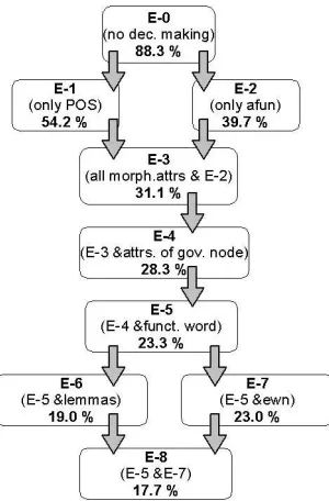
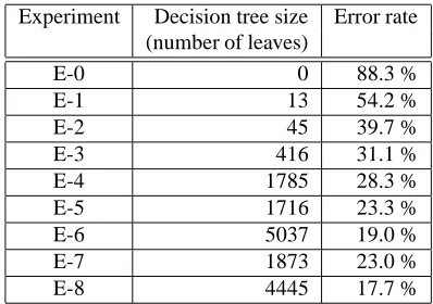
In order to find the importance of individual attributes for the overall performance, the system was trained repeat-edly using different sets of input attributes. The experi-ments can be ordered into a lattice according to the sub-sumption of their attribute sets (Figure 4). In the follow-ing paragraphs, the experiments will be evaluated one by one and associated with an illustrative example of a rule acquired by C5. You can also see Table 1 for the evaluation summary.
Not only the sequence of experiments shows the contri-bution of different attributes to the performance, but it can also demonstrate the process of acquiring more “clever” rules.
E-0) No input attributes
The first experiment functions only as a baseline, because no attributes were used for decision and no decision tree was generated. Every node in the testing set was simply assigned with the most frequent functor from the training set. The resulting error rate is 88.3 %.
Figure 4: The lattice depicts the subsumption of attribute sets within the sequence of experiments, and the impact of enlarging the attribute set on the resulting error-rate.
E-1) Input attributes: part of speech of node N
Error rate: 54.2%
Decision tree size: 13 leaves Sample from the ruleset:
Rule 7: (3584/461, lift 4.0) d pos = A
-> class RSTR [0.871]
Possible interpretation of the rule: An adjective usually is the restrictive adjunct.
E-2) Input attributes: analytical function of given node.
Error rate: 39.7%
Decision tree size: 45 leaves Sample from the ruleset:
Rule 21: (2244/323, lift 5.5) d_afun = Sb
-> class ACT [0.856]
Interpretation: The subject of a sentence usually be-comes its actor.
E-3) Input attributes: morphological attributes and an-alytical function of given node.
Error rate: 31.1%
Decision tree size: 416 leaves Sample from the ruleset:
Rule 213: (251/130, lift 29.2) d_case = 3
d_afun = Obj
-> class ADDR [0.482]
Interpretation: An object in dative becomes addressee.
E-4) Input attributes: morphological attributes and an-alytical function of given node and of its autosemantic governor G
Error rate: 28.3%
Rule 388: (16/4, lift 4.7) g_voice = P
d_case = 7 d_afun = Obj
-> class ACT [0.722] Rule 665: (137/14, lift 5.9)
g_voice = P d_afun = Sb
-> class PAT [0.892]
Interpretation: The subject in a clause in passive voice becomes patient, the actor is expressed by instrumental (Compare with the rule in E-2).
E-5) Input attributes: Same attributes as in E-4, but lemmas of functional word (prepositions, conjunctions) were added.
Error rate: 23.3%
Decision tree size: 1716 leaves Sample from the ruleset:
Rule 11: (63/16, lift 108.0) d afun = Adv
preposition = s -> class ACMP [0.738] Rule 174: (16, lift 231.1)
d afun = Adv
subord conj = protoˇze -> class CAUS [0.944] Rule 412: (34/6, lift 368.7)
coord conj = nebo -> class DISJ [0.806]
Interpretations: (i) A node connected via preposition s (‘with’) represents accompaniment. (ii) A clause connected via subordinating conjunction protoˇze (‘because’) relates to causality. (iii) A coordination node with lemma nebo (‘or’) expresses disjunction.
E-6) Input attributes: same attributes as in E-5, but lemmas of both nodes were added.
Error rate: 19,0%
Decision tree size: 5037 leaves Sample from the ruleset:
Rule 511: (40, lift 28.6) d lemma = rok
preposition = v
-> class TWHEN [0.976] Rule 1031: (6/3, lift 3.2)
g lemma = ˇcinnost d pos = N
preposition = empty -> class ACT [0.500] Rule 617: (11, lift 736.0)
d lemma = dosud
-> class TTILL [0.923] Rule 1397: (6, lift 71.6)
g lemma = patˇrit preposition = mezi -> class DIR3 [0.875]
Interpretation: (i) v roce (‘in year’) is temporal modifier. (ii) A noun directly depending on noun ˇcinnost (‘activity’) is probably actor of the activity. (iii) dosud (‘still’, ‘untill now’) is a temporal modifier (TTILL - ‘time till . . . ’). (iv)
patˇrit mezi . . . (‘belong between . . . ’) binds a directional
modifier.
Note: Rules like 1031 and 1397 can be understood as a pro-jection of the behavior of nouns and verbs on the treebank data.
E-7) Input attributes: morphological attributes and an-alytical function of node N
Error rate: 23.0%
Decision tree size: 1873 leaves Sample from the ruleset:
Rule 237: (115, lift 29.0) d_afun = Adv preposition = v d_ewn_time = yes
-> class TWHEN [0.991]
Interpretation: An adverbial formed by a noun that has (according to EuroWordNet) something to do with time and that is connected via preposition v (‘in’), is a temporal mod-ifier of type TWHEN.
E-8) Input attributes: union of attributes from E-6 and E7
Error rate: 17.7%
Decision tree size: 4445 leaves Sample from the ruleset:
Rule 70: (4, lift 132.9) g lemma = mnoˇzstv´ı d ewn origin = yes -> class MAT [0.833]
Interpretation: If an item depends on noun mnoˇzstv´ı (‘amount’) and it is related to concept Origin in EuroWord-Net, then it has the functor MAT (material, e.g. amount of wood).
3.3. Further Observations
Experiment Decision tree size Error rate (number of leaves)
E-0 0 88.3 %
E-1 13 54.2 %
E-2 45 39.7 %
E-3 416 31.1 %
E-4 1785 28.3 %
E-5 1716 23.3 %
E-6 5037 19.0 %
E-7 1873 23.0 %
E-8 4445 17.7 %
Table 1: Evaluation of the sequence of experiments.
3.3.1. Robustness
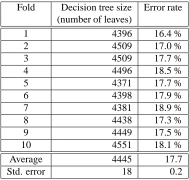
Table 2 shows the evaluation of experiment E-8 for each fold separately. The error-rate varies only in a narrow in-terval from 16.4 % to 18.1 %. This observation guarantees satisfactory robustness of the system.
Fold Decision tree size Error rate (number of leaves)
1 4396 16.4 %
2 4509 17.0 %
3 4509 17.7 %
4 4496 18.5 %
5 4371 17.7 %
6 4398 17.9 %
7 4381 18.9 %
8 4438 17.3 %
9 4449 17.5 %
10 4551 18.1 %
Average 4445 17.7
Std. error 18 0.2
Table 2: Evaluation of experiment E-8 on the individual folds of 10-fold cross-validation.
3.4. Error-rate versus training data size
In order to examine the dependence of the error-rate on the data set size, the experiment E-8 was repeatedly per-formed for data sets containing 1 %, 3 %, 6 %, 10 %, 30 %, and 60 % of all available data. The resulting values of error-rate, as well as the curve interpolated from them, are depicted in Figure 5. The curve tends to go down even in its last segment, which is promising. If we extrapolate the curve, a decrease of the error-rate by several percent-age points can be expected when the size of the data set reaches 100 000 nodes. On the other hand, the “speed of the improvement” of the presented system decreases too fast, therefore it is not likely that its error-rate can ever drop under 10 % using the same attribute set and the same ML technique.
Although this observation perhaps seems to be pes-simistic, it perfectly matches the fact that if two human annotators are asked to annotate (independently on each other) the same sentences, roughly 10 % of the functors differ (Hajiˇcov´a et al.,2002). A part of the disagreements is naturally caused by human errors. However, there are probably also certain classes of problems, which are caused by the fact that the present annotation scheme cannot fully capture the vagueness of the language. In any case, the per-centage of functors on which two people differ, makes a natural limit for what is called error rate in this paper.
4.
Accelerating the Annotation Process
4.1. Annotation Environment
For the tectogrammatical annotation of the PDT, the an-notators use a special Tree Editor (TrEd for short). It en-ables a comfortable and fast handling of the topology of the trees (correction of “wrongly-aimed” dependencies) as well as node re-labeling (changing node attributes, espe-cially functors). More details can be found in (Hajiˇc et
Figure 5: The improvement of the error-rate when increas-ing the size of the trainincreas-ing data (the attribute set is identical with that of E-8). The data size is expressed as the number of vectors (edges). The dashed line represents the average degree of “disagreement” between two human annotators. .
Figure 6: An illustration of the Tree Editor - the soft-ware tool for the manual annotation on the tectogrammati-cal level.
al.,2001). The user interface of TrEd is depicted in Fig-ure 6.
4.2. Incorporation of the Decision Trees into the Annotation Process
In order to make the presented system for functor as-signment practically usable, it has to be incorporated into the annotation process. This is done as follows: the deci-sion tree generated by C5 is (automatically) translated into a module in Perl (the programming language TrEd is writ-ten in). In TrEd, a keyboard shortcut is defined which ex-ecutes the evaluation of the decision tree subsequently for each node of the tectogrammatical tree, and it assigns func-tors to these nodes.
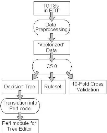
deci-Figure 7: Data flow diagram. An the beginning, there is a set of manually annotated tectogrammatical tree structures. At the end, a Perl module for automatic functor assignment is created and can be “plugged” into the tree editor.
sion tree. We color the automatically assigned functors ac-cording to the confidence of the applied leaf of the decision tree, with the intent to make it easier for annotators to focus their concentration on the most “suspicious” nodes. Red is used for functors with estimated confidence lower than 60 %, black for confidence higher than 90 %, and blue for the rest. If an annotator corrects the automatically assigned functor, its color changes to green (the annotator can then easily perceive which functors have already been manually corrected).
4.3. Response of the Human Annotators
Currently, there are six people who have been manually annotating the tectogrammatical tree structures for at least one year. All of them have more than half a year of expe-rience with using AFAS. They were given a questionnaire, the goal of which is to determine the real usefulness of the AFAS. Here we present selected results of this inquiry.
All of the annotators share the opinion that the AFAS significantly increases the speed of their work. Ac-cording to their subjective estimate, the manual as-signment of functors would take at least twice as long without the AFAS.
As it was already mentioned in this paper, they were asked whether they prefer to automatically assign only functors with high confidence, or to assign as many functors as possible, even though more errors would occur (precision versus recall question). All of them chose the latter possibility.
They were also asked whether they find the coloring (expressing the confidence of functors) useful. Ac-cording to their answers, it unfortunately seems that they are not using this information at all, even though
on unseen data at least 75 % of errors are among “red” functors. They check the whole tree node by node for each sentence and cannot simply skip over some parts.
They were asked whether they are aware of any sys-tematical error made by the AFAS. One of their sug-gestions actually resulted in a change of the input at-tribute set used by the AFAS (topological atat-tributes have been added).
4.4. Error Analysis
Having in hand the files during the annotation of which the previous version of the AFAS was used, we can eval-uate how often the automatically assigned functors were manually corrected. The resulting number of corrections (roughly 23 %) nearly exactly matches the predicted error-rate, which again confirms the robustness of this approach. For one file (53 sentences), the errors were analyzed in detail. In this way, we try to localize the bottlenecks of the system: the most frequent types of misclassification, and (if possible) the most frequent reasons for such misclassifi-cation. Such observation are leading us to furher improve-ments.
5.
Conclusion
We have shown that the machine learning approach can be very helpful during the tectogrammatical annotation of the Prague Dependency Treebank, even though such anno-tation is very close to the semantics of natural language. Only roughly one out of five automatically assigned func-tors has to be manually corrected, which makes the remain-ing annotation significantly faster in comparison with an-notation from scratch. It is also interesting that the number of differences between manually assigned functors and au-tomatically assigned functors is less than twice as big as the number of differences between two humans.
We hope that further improvements of the presented systems will be reached via (i) larger training data, (ii) er-ror analysis of misclassifications of the existing system, (iii) newly available lexical resources (especially a valency lex-icon of Czech verbs (Lopatkov´a, ˇZabokrtsk´y,2002)).
Acknowledgements
The research reported on in this paper has been car-ried out mainly under the projects GA ˇCR 405/96/K214 and M ˇSMT LN00A063. The authors also gratefully acknowl-edge the support from ILPNet2.
6.
References
S. Dˇzeroski, Z. ˇZabokrtsk´y. 2001. A Machine Learning Ap-proach to Automatic Functor Assignment in the Prague Dependency Treebank. Prague Bulletin of Mathematical
Linguistics, 76: 35–43. Charles University, Prague.
J. Hajiˇc. 1998. Building a syntactically annotated corpus: The Prague Dependency Treebank. In: Issues of Valency
and Meaning. Studies in Honour of Jarmila Panevov ´a,
ed. by E. Hajiˇcov´a, 106-132. Karolinum, Prague. J. Hajiˇc, P. Pajas, B. Hladk´a. 2001. The Prague Dependency
Treebank: Annotation Structure and Support, In:
Pro-ceedings of the IRCS Workshop on Linguistic Databases,
E. Hajiˇcov´a. 2002. Dependency based underlying-structure tagging of a very large Czech corpus. In: Les grammaires
de dpendance. Traitement Automatique des Langues 41,
ed. by Sylvain Kahane, 57-78.
E. Hajiˇcov´a, P. Pajas, E. Vesel´a. 2002. Consistency in Deep Syntactic Annotations of Corpora: The Case of PDT. Submitted at The 19th International Conference on
Com-putational Linguistics.
Hajiˇcov´a, E., Panevovov´a, J., Sgall, P., 1999. Manual for tectogrammatical annotation. Technical Report
UFAL-TR-7. Charles University, Prague
E. Hajiˇcov´a, B. H. Partee, P. Sgall. 1998. Topic-focus, tripartite structures and cognitive content. Dordrecht: Kluwer.
M. Lopatkov´a, Z. ˇZabokrtsk´y. 2002. Valency Dictionary of Czech Verbs: Complex Tectogrammatical Annotation. In: Proceedings of Third International Conference on
Language Resources and Evaluation. Las Palmas, Spain.
J.R. Quinlan. 1993. C4.5: Programs for Machine Learning. Morgan Kaufmann, San Mateo, CA.
Z. ˇZabokrtsk´y. 2000. Automatic Functor Assignment in the Prague Dependency Treebank. In Proceedings of the
Third International Workshop on Text, Speech and Dia-logue. Springer, Berlin.
Appendix
Alphabetically Ordered List of 40 Most Frequent Functors
ACMP (accompaniement): mothers with children ACT (actor): Peter read a letter.
ADDR (addressee): Peter gave Mary a book.
ADVS (adversative): He came there, but didn’t stay long. AIM (aim): He came there to look for Jane.
APP (appuerenance, i.e., possesion in a broader sense): John’s desk
APPS (apposition): Charles the Fourth, (i.e.) the Emperor ATT (attitude): They were here willingly.
BEN (benefactive): She made this for her children. CAUS (cause): She did so since they wanted it. COMPL (complement): They painted the wall blue. COND (condition):If they come here, we’ll be glad. CONJ (conjunction): Jim and Jack
CPR (comparison): taller than Jack
CRIT (criterion): According to Jim, it was rainng there. DENOM (denomination): Chapter 5 (e.g. as a title) DIFF (difference): taller by two inches
DIR1 (direction-from): He went from the forest to the
village.
DIR2 (direction-through): He went through the forest to
the village
DIR3 (direction-to): He went from the forest to the village. DISJ (disjunction): here or there
DPHR (dependent part of a phraseme): in no way, gram-mar school
EFF (effect): We made him the secretary. EXT (extent): highly efficient
FPHR (foreign phrase): dolcissimo, as they say ID (entity): the river Thames
LOC (locative): in Italy
MANN (manner): They did it quickly. MAT (material): a bottle of milk MEANS (means): He wrote it by hand. MOD (mod): He certainly has done it.
PAR (parentheses): He has, as we know, done it yesterday. PAT (patient): I saw him.
PHR (phraseme): in no way, grammar school
PREC (preceding, particle referring to context): therefore, however
PRED (predicate): I saw him. REG (regard): with regard to George
RHEM (rhematizer, focus sensitive particle): only, even, also
RSTR (restrictive adjunct): a rich family
THL (temporal-how-long ): We were there for three
weeks.