Feature Weighting Random Forest for Detection of Hidden Web Search Interfaces

(1)

(2)

(3)

(4)

390 Yunming Ye et al.

The rest of this paper is organized as follows. In Section 2, we formalize the detecting search interface problem as a form classification problem and present the feature extraction techniques. Section 3 describes the improved random forest algorithm for form classification. Experimental results and analysis are presented in Section 4. Section 5 concludes this paper and presents our future work.

2. Feature Extraction for Form Classification

Search interface detection is a process of distinguishing the search forms of the hidden Web from non-search forms. It is a two-class classification problem in machine learning. This section describes how to extract form features from HTML pages and discusses the characteristics of the data matrix for form classification.

2.1 Feature Extraction Rules

An HTML form usually begins with the tag <FORM> and ends with the tag < /FORM >. According to this rule, HTML forms can be extracted by searching the <FORM > tag in HTML pages. Each extracted form is a sample in the training set. The features of each form are generated by parsing the corresponding <FORM> HTML block.

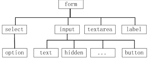
HTML forms contain two kinds of features: one is the attributes of forms and elements, and the other is the statistics of those attributes. A form mainly contains four kinds of elements, that is, “INPUT”, “SELECT”, “LABEL” and “TEXTAREA”, which are the children elements of “FORM” element. Element “INPUT” contains several types, such as “text”, “hidden”, etc. The hierarchy of a form is shown in Figure 1. All of these elements contain a set of attributes, such as “name”, “value”, “size”, etc. The attributes of “form” elements are “method”, “action”, and “name”. Attribute “method” indicates the method for the form to submit query data, such as “POST” or “GET”. Attribute “action” indicates the address of the corresponding server of the form, and attribute “name” indicates the name of the form. Some elements and attributes can be removed because they are not useful for form classification, for instance “option”, “size”, “width”, etc. Besides, the statistics about the number of elements or attributes in each element can also be computed as important features.

(5)

Feature Weighting Random Forest for Detection of 391 Hidden Web Search Interfaces

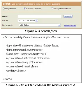
Figure 2 shows an example of a search form. The form contains three elements: one “SELECT” element and two “INPUT” elements. There are three attributes in the “SELECT” element : “name” with value “and”, “size” with value “1”, and “width” with value “50”. It also contains several “OPTION” elements. The “size” and “width” attributes, along with the “OPTION” elements are not useful for form classification, so they can be removed. The corresponding HTML codes are shown in Figure 3.

Figure 2. A search form

Figure 3. The HTML codes of the form in Figure 2

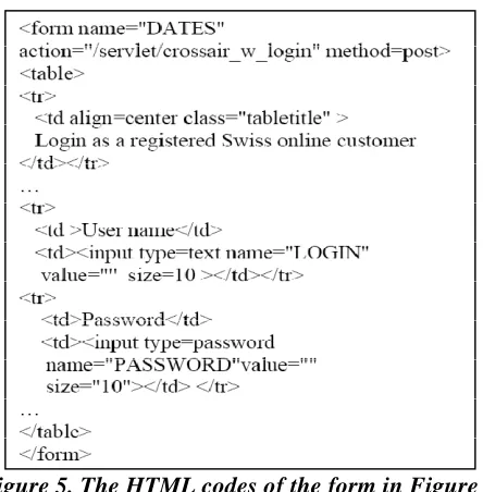
Figure 4 shows an example of a non-search form. The corresponding HTML codes are shown in Figure 5. According the feature extraction rules, the useful form elements in this form include “INPUT”, “LABEL”, and “FORM”, which can be used to compose the feature space. Elements “TABEL”, “FONT”, and “TR” can be removed because they are not useful.

(6)

Figure 5. The HTML codes of the form in Figure 4

There are some important differences between the features of search form and non-search form. First, the number of “INPUT”, “SELECT”, and “TEXTAREA” elements in search forms is larger than that in non-search forms. Second, the value of the “method” attribute in “FORM” elements is always set as “POST” in search forms, while it is always set as “GET” in non-search forms. Moreover, the elements’ values of search forms often contain some keywords such as “search”, “find”, or other words that have the same meaning as “search”. These differences, however, are not the only decisive factors. There are other features that can be explored by classification algorithms.

According to the major differences, six kinds of rules are used in the feature extraction process as follows:

1. Extract the “name” attribute values from “input”, “select”, “textarea”, and “label” elements;

2. Extract the “value” attribute value from “input”, “textarea”, and “label” elements; 3. Extract the “name” and “method” attribute values from “form” elements;

4. Extract the words that appear between slashes(/) in the “action” attributes of the “form” elements;

5. Extract the words that appear between slashes(/) in the “src” and “alt” attributes of the “input-image” element;

(7)

(8)

(9)

(10)

Algorithm 1 The pseudo-code of the feature weighting random forest algorithm

Input:

- D: the training database (its number is d ),

- N: the features of the forms (its number is n), -

C

: the target class attribute C=yes no, ,

- k: the number of decision trees,

- β: the selection rate of features.

Output: the decision forest M∗.

Process:

1. Compute the weight W based on Formula (1); 2. Sort N on the descending order of weight W;

3. Let n′ =_⎣⎢β⋅n_⎦⎥, and select ⎢_⎣β⋅n⎥_⎦ features with larger weights as the training samples; 4. for i=1 to kdo

(a) Select d′samples from the training samples by bootstrapping;

(b)Randomly select tfeatures; where t=_⎣⎢log₂n′+1⎥_⎦and the selection is biased towards the features with larger weights;

(c) Build a decision tree from the d′samples with selected features;

(d) Add the learned decision tree to M∗; endfor

5. Using M∗to do classification based on Formula (4).

3.3 The computational complexity

The computational complexity of RFA (Breiman, 2001) is O ktd( log )d , where kis the

number of decision trees, t is the number of attributes, d is the number of training samples.

In IRFA, the enumerating number of the feature attribute is constant (Formula (1)). The computational complexity of all feature weights is ( )O n . Using the bucket sorting method, the weights can be sorted in linear time. Therefore, the computational complexity of the IRFA is O ktd( logd+αn), where t=_⎣⎢log₂n+1⎥_⎦. Therefore, the computational complexity of IRFA is very close to the complexity of RFA.

The computational cost depends on three factors: the number of decision trees k, the

number of features n, and the number of training samples d. We will discuss how to select

(11)

4. Experiments

4.1 Data Sets

We used two Web page collections in our experiments. One was taken from project Metaquerier1_{, and the other was created by crawling the website Search Engine Guide}2_{with a} Web crawler implemented in Java. The two collections represent a pseudo-random crawling of the Web. A HTML parser was developed to extract the HTML forms and their context features from these two collections. The extracted forms were used to compose the final data sets for experiments.

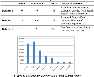
Table 3. The three data sets used in the experiments

search non-search features content of data sets

Data set 1 46 43 198

Extracted from the website collection crawled from Search Engine Guide by crawler

Data Set 2 65 116 208

Extracted from artificial website collection of Metaquerier project

Data Set 3 51 96 202 The forms are selected from _{data set 1 and data set 2.}

Figure 6. The domain distribution of non-search forms

We manually classified the extracted forms into search forms (i.e., real search interface of hidden Web) and non-search forms. Three classification data sets were constructed from the classified forms, as shown in Table 3. The three data sets have a variety of sample distributions. Data set 1 and Data set 2 cover different domains, while Data set 3 is a mixture

(12)

of the two domains. The three data sets also have different feature types and feature numbers. The average number of features in the data sets is over 200, while the average number of samples is less than 140. The matrices of the three data sets were quite sparse, and the number of features was quite large.

To further test the robustness of our method, the non-search forms in the data sets were made of a variety of forms, including registration forms, login forms, network investigation forms, etc. Figure 6 shows the distribution of different non-search forms.

4.2 Comparison Experiments

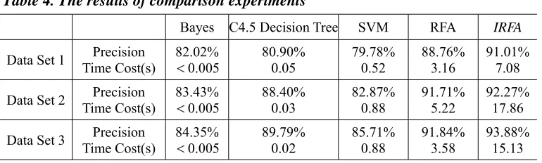
We first carried out experiments to compare our random forest method with four well-known classification algorithms, i.e., Support Vector Machine (SVM), C4.5, Naïve Bayes,and Random Forest Algorithm (RFA) implemented in Weka3_{. We also implemented our algorithm} (IRFA) as a plug-in of Weka and conducted all experiments in this environment to make a fair comparison. We conducted the standard 10-fold classification experiments on the three data sets. The evaluation metrics used were precision and computation time. The number of trees was set to 100 for IRFA and parameter β set to 0.5 . The final experimental results are shown in Table 4.

Table 4. The results of comparison experiments

Bayes C4.5 Decision Tree SVM RFA IRFA

Data Set 1 _{Time Cost(s)}Precision 82.02% _<_0.005 80.90% _0.05 79.78% _0.52 88.76% _3.16 91.01% _7.08 Data Set 2 _{Time Cost(s)}Precision 83.43% _<_0.005 88.40% _0.03 82.87% _0.88 91.71% _5.22 92.27% _17.86 Data Set 3 _{Time Cost(s)}Precision 84.35% _<_0.005 89.79% _0.02 85.71% _0.88 91.84% _3.58 93.88% _15.13 We can see that IRFA showed significant improvement over the other four algorithms. The result of C4.5 was better than SVM and Naïve Bayes. This was due to the fact that there were a lot of missing values in the data sets and SVM and Naïve Bayes did not perform well in this kind of sparse data. The high dimensionality in the training sets, however, causes an overfitting problem to C4.5 because the single decision tree could become very complex. RFA and IRFA can avoid this problem by selecting different subsets of features to build individual decision trees. Compared with RFA, IRFA uses features that are more correlated to the class label feature, so the accuracy of each individual tree is improved. Therefore, our method got better performance than RFA. Since IRFA needed to compute the χ2 values for features, it

(13)

took more computational time. This extra overhead, however, is worthwhile and acceptable in real applications because the training process is offline and not executed frequently.

4.3 Selection of the Number of Features

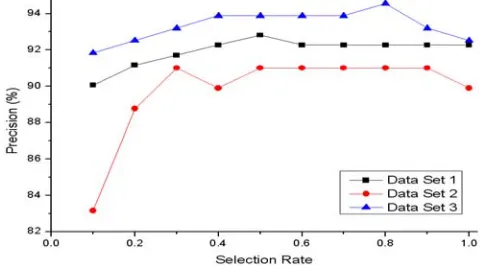
When building each decision tree, IRFA only selects a subset of the original features. The number of selected features is controlled by the selection rate β. Different selection rates result in different classification precisions and computational costs. We carried out experiments on the three data sets with β =0.1, 0.2, , 1.0… . Figure 7 plots selection rate β

against precision, while Figure 8 is β against computational cost.

Figure 7 shows that when β <0.5, the precision increases greatly as the selection rate increases. The reason is that a larger selection rate increases the number of features to be selected. When 0.5≤β ≤0.8, the classification performance becomes relatively stable. This means that the forest has selected enough discriminative features. When β >0.8, the precision will decrease as the selection rate increases. This can be explained by the idea that having too large a selection rate will increase the possibility of selecting noisy features. Most experiments have shown that β =0.5 was a good setting.

Figure 8 shows that the computational time of IRFA increases linearly as the feature selection rate increases. This property indicates that IRFA is scalable to large high-dimensional data.

Figure 7. Influence of the number of features on precision

(14)

4.4 Selection of the Number of Trees

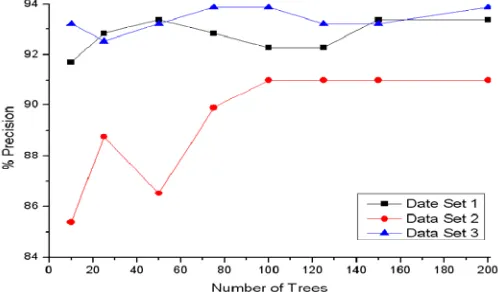
Another interesting issue is whether the performance of IRFA highly depends on the size of a forest (number of decision trees in the forest). Since a large number of trees lead to a considerable computational cost, we need to find a good tradeoff between classification precision and computational cost. We performed experiments on the three data sets with different tree numbers (k=10, 25,50,75,100,125,150, 200). The feature selection rate β was set to 0.5 in all experiments. The experimental results are shown in Figure 9 and Figure 10.

Figure 9 plots the precision against the number of trees k. The results show that if the number of trees is too small, the classification performance of the forest will be unstable. If the number of trees is too large, however, the computational cost for generating a forest will be very high. The classification precision becomes stable when 75< <k 150 . The near-optimal precision can be obtained when k is set to 100. Moreover, as shown in Figure 10, with the increase of the number of trees, the computational time increases linearly as well. Therefore, in most situations, k=100 is a good balance between classification accuracy and computational cost.

Figure 9. Influence of the number of trees on precision

(15)

(16)

is attained by computing the difference between the prior uncertainty and expected posterior uncertainty using X . Feature X is preferred to feature Y if the information gain from

feature X is greater than that from feature Y (Dash & Liu, 1997). In this experiment, the

information gain from feature X is set to feature X as its weight instead of Chi-square

value in IRFA.

3. Gain Ratio is an extension of information gain. It attempts to overcome the problem that the information gain measure is biased toward tests with many outcomes (i.e., it prefers to select attributes having a large number of values) (Han & Kamber, 2007). The process of embedding gain ratio into IRFA is similar to information gain in our experiment.

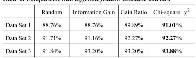
4. Chi-square χ2 that has been explained in Section 3.2. The experiments in the prior sections were all based on this feature selection method.

Table 6. Comparison with different feature selection schemes

Random Information Gain Gain Ratio Chi-square χ2

Data Set 1 88.76% 88.76% 89.89% 91.01%

Data Set 2 91.71% 91.16% 92.27% 92.27%

Data Set 3 91.84% 93.20% 93.20% 93.88%

We implemented the four feature selection methods in Weka’s random forest package, and carried out experiments on the data sets described in Section 4.1. The results are shown in Table 6. From the results, we can see that the Chi-square method is better than the others. The reason that Information Gain and Gain Ratio scheme did not attain better performance can be explained as follows: since both of them use the same feature evaluation criterion in feature sampling and tree construction (for node splitting), the information of features cannot be fully exploited.

5. Conclusions

(17)

(18)

Larson, H. J. (1982). Introduction to probability theory and statistical inference. New York: Wiley, 3 ed.

Ntoulas, A., Zerfos, P., & Cho, J. (2005). Downloading textual hidden web content through keyword queries.

Quinlan, J. R. (1993). C4.5: Programs for Machine LearningMachine Learning. Morgan Kaufmann.

Raghavan, S., & Garcia-Molina, H. (2001). Crawling the hidden web. Proceedings of the 27th International Conference on Very Large Data Bases. Roma, Italy.

Wang, J., & Lochovsky, F. (2003). Data extraction and label assignment for web databases. Proceedings of the 12th International World Wide Web Conference. Budapest, Hungary. Zhang, Z., He, B., & Chang, K. C. (2004). Understanding web query interfaces: best-effort