Weighted maximum likelihood as a convenient shortcut to optimize the
F-measure of maximum entropy classifiers
Georgi Dimitroff, Laura Tolos¸i, Borislav Popov and Georgi Georgiev Ontotext AD, Sofia, Bulgaria
georgi.dimitrov, laura.tolosi, borislav.popov, [email protected]
Abstract
We link the weighted maximum entropy and the optimization of the expectedFβ
-measure, by viewing them in the frame-work of a general common multi-criteria optimization problem. As a result, each solution of the expectedFβ-measure
max-imization can be realized as a weighted maximum likelihood solution - a well un-derstood and behaved problem. The spe-cific structure of maximum entropy mod-els allows us to approximate this charac-terization via the much simpler class-wise weighted maximum likelihood. Our ap-proach reveals any probabilistic learning scheme as a specific trade-off between dif-ferent objectives and provides the frame-work to link it to the expectedFβ-measure.
1 Introduction
In many NLP classification applications, the classes are not symmetric and the user has some preference towards a high Precision or Recall of a particular target class. Thus, appropriate tun-ing of the model is often necessary, dependtun-ing on the particular tolerance of the application to false positive or false negative results. This pref-erence can be expressed by requiring a large Fβ
measure for a particularβ describing the desired Precision/Recall trade-off. Ideally, the parameters of the linear model should be estimated such that a desired Fβ measure is maximized. However,
directly maximizing Fβ is hard, due to its
non-concave shape.
Maximum likelihood-based classifiers such as the maximum entropy are relatively easy to fit,
but they are rigid and cannot be tuned to a de-sired Precision and Recall trade-off. In this ar-ticle, we consider a more flexible maximum en-tropy model, which optimizes a weighted likeli-hood function. If appropriate weights are chosen, then the maximum weighted likelihood model co-incides with the optimalFβmodel. The advantage
of the weighted likelihood as a loss function is that it is concave and standard gradient methods can be used for its optimization. In fact an existing maxi-mum entropy implementation can be easily gener-alized to the weighted case.
To the best of our knowledge, such a link be-tween the maximum likelihood and theFβhas not
been established before. The article is focused on the intuition of the relation and the sketch of the proof of the main result. We also present numeri-cal experiment supporting the theoretinumeri-cal findings. Additional value of our theoretical observation is that it establishes the methodology of viewing a particular probabilistic model as a specific solu-tion of a common multi-criteria optimizasolu-tion prob-lem.
This article is organized as follows. In Sec-tion 2 we present related work, SecSec-tions 3 to 6 present the theoretical aspects of link between the weighted maxent andF measure. Section 7 intro-duces the algorithm, Section 8 explains the steps for evaluation of the algorithm, Section 9 presents the datasets. Sections 10 and 11 present aspects of performance of our method on the datasets and Section 12 concludes the paper.
2 Related work
The most popular heuristic for Precision-Recall trade-off is based on adjusting the acceptance threshold given by maximum entropy models (or
Algorithm 1Golden Section Search
Require: Unimodal functionf, interval[a, b] Ensure: x∗= arg maxxf(x)
1: φ←1+√5 2
2: functionGSS(f,a,b,p1,p2) 3: if|b−a|< εthen 4: returna
5: else
6: iff(p1)> f(p2)then
7: b←p2
8: p2←p1
9: p1←(2−φ)(b−a)
10: else
11: a←p1
12: p1←p2
13: p2←(2−φ)(b−a)
14: end if
15: returnGSS(f, a, b, p1, p2)
16: end if 17: end function
18: p1←a+ (2−φ)(b−a)
19: p2←b−(2−φ)(b−a)
20: x∗←GSS(f, a, b, p1, p2)
are described in the Results section.
First, we evaluated Precision and Recall at dif-ferent values of the class weightwin the interval
[0.1,5]and show that they are antagonistic, which demonstrates that weighted maxent can trade-off Precision and Recall.
Second, we show that our golden section search algorithm finds a good approximation of the op-timum class-weightw, necessary for maximizing a specificFβ(w), despite the violation of the
uni-modality ofFβ(w). We can identify the optimum
weights by means of a brute-force approach, by which we try a large number of values for the weight of the target class (in practice, 50 values evenly distributed in [0.1,5]). The brute-force
is infeasible practical applications, because it re-quires training a large number of weighted max-ent models. The comparison to the brute-force
method is carried on the training set, because find-ing the appropriate class weightwis part of model fitting, together with the estimation of the model weightsλ.
Third, we demonstrate that the models that we fit are superior (i.e. yield better testFβ) than the
maxent model. To this end, we computeFβ for a
range of values ofβ ∈ [0,1]. We compare these results with the test Fβ that our algorithm
deliv-ers. For a reliable comparison, we also estimate the variance of theFβvalues – both for our method
and for the baseline – by training on20bootstrap samples of the training set instead of the original
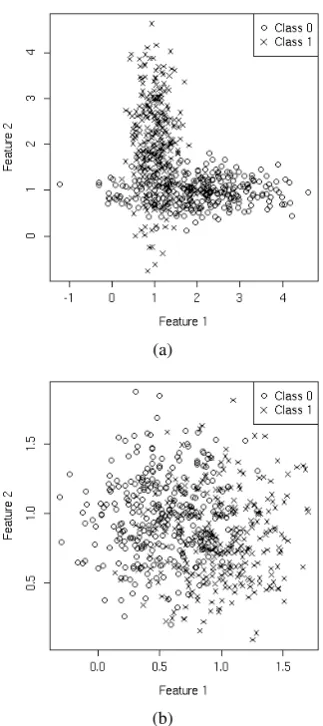
(a)
(b)
Figure 1: Distribution of the samples in the space of fea-tures for the synthetic datasets: a) dataset A ; b) dataset B
train set.
9 Datasets
9.1 Synthetic datasets
We simulated two datasets, A and B, of 600
samples each of them with two equally popu-lated classes and only two features. In dataset A the samples from class 0 are distributed as
N(µA0,ΣA0), with µA0 = (2,1) and ΣA0 = (1,0.3)>I2. Class1is generated byN(µA
1,ΣA1), withµA1 = (1,2)andΣA1 = (0.3,1)>I2.
Dataset B consists of two symmetric spheri-cal Gaussians -N(µB
0,ΣB0)andN(µB1,ΣB1)with µB0 = (0.5,1), ΣB0 = (0.3,0.3)>I2, µB1 = (1,0.8)andΣB1 = (0.3,0.3)>I2.
In Figure 1 we visualize both synthetic datasets. We used400of the samples for training and200
9.2 Twitter sentiment corpus
We used the Sanders Twitter Sentiment Cor-pus (http://www.sananalytics.com/lab/twitter-sentiment/), from which we filtered3425 tweets, labeled as either positive, negative or neutral. We classified tweets that expressed a sentiment (either positive or negative), versus neutral tweets. The neutral tweets are about twice more than the positive and negative tweets together. For the experiments, we used3081(90%) tweets for train-ing and343(10%) for testing. We processed the tweets and obtained about6095features. In order to avoid overfitting and speed up computations, we used a filter method based on Information Gain to remove uninformative features. We kept
60(10%) of the features for our experiments.
10 Experiments and results
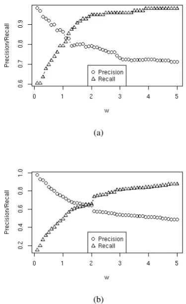
By varying the weight of the target class, the weighted maximum entropy achieves Precision-Recall trade-off. Figure 2 clearly illustrates the trade-off, for the synthetic data A and the twitter sentiment data. Additionally, note that Precision and Recall are in equilibrium for a a weight that reflects the ratio of the class cardinalities, namely w = 1 for the balanced synthetic dataset A and w= 2, for the twitter corpus.
Thebrute forcemethod reveals the shape of the Fβ(w), as a function ofβ andw(see Figure 4 a)
and c)). Both of our datasets suggest that there is a critical value of wwhich marks a switch point in the monotony of theFβ(w)(regarded as a
func-tion ofβ). Forwsmaller than the critical switch, Fβ(w)increases withβ, and forwlarger than the
switch, Fβ(w) decreases with β. This switch is
probably directly related to the ratio of the class cardinalities and deserves further theoretical in-vestigation.
Figures 4 a) and c) show also the ‘path’ that marks the maximumFβ achievable for eachβ, in
solid black line. The path corresponding to our golden search algorithm falls fairly close to that of the brute force, as shown by the dotted lines (marking the mean and one standard deviation to each side). Even if sometimes the optimalwis not found exactly by the golden search, theFβ is still
very close to the optimum, as shown in Figures 4 b) and d). In fact, the optimumFβis always within
one standard deviation from the expected value of our golden search algorithm.
Finally, we demonstrate that our method
per-(a)
(b)
Figure 2: Precision-Recall trade-off on the train set by changing class-weights: a) synthetic dataset A; b) sentiment tweeter dataset.
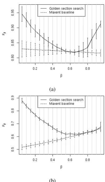
forms very well on the test set, compared to the simple maxent baseline. Figure 3 a) and b) show that the testFβ is superior to the baseline, due to
its ability to adapt the fitted model to the specific Precision - Recall trade-off, expressed by a value ofβ.
11 Limits and merits of the weighted maximum entropy
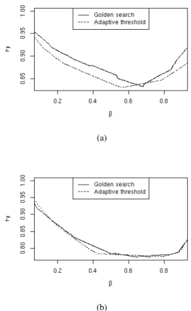
In this section we compare the weighted maximum entropy and the acceptance threshold method with the help of the two artificial data sets A and B shown on Figure 1. The acceptance threshold cor-responds to a translation of the separating hyper-plane obtained by the standard maximum entropy model. We show that acceptance threshold fails to fit the data well for most values ofβ, if the data resemble more dataset A than dataset B. In con-trast, the weighted maxent is more adaptive, fitting nicely both datasets for all values ofβ.
(a)
(b)
Figure 3:TestFβfor our method, compared to the maxent baseline. One standard deviation bars are added. a) synthetic data; b) twitter corpus.
the synthetic data set B. Indeed, Figure 5 b) shows that the acceptance threshold and the weighted maximum entropy do result in virtually the same optimalFβvalues.
The optimal Precision/Recall trade-off for dataset A however requires additional rota-tion/tilting of the separating hyperplane that can-not be produced by adjusting the acceptance threshold. In line with this intuition Figure 5 a) demonstrates that the weighted likelihood settles at a better Precision-Recall pairs and consequently results in largerFβ values.
Clearly, in the general case the optimal shift of the separating plane is expected to have a rotation component that is unaccessible by simply adjust-ing the acceptance threshold.
12 Conclusion and future work
The main result of the paper is that the weighted maximum likelihood and the expected Fβ
mea-sure are simply two different ways to specify a particular trade-off between the objectives of the same multi-criteria optimization problem. Techni-cally we unify these two approaches by viewing them as methods to pick a particular point from
(a)
(b)
(c)
(d)
(a)
(b)
Figure 5: Comparison of the acceptance threshold versus the weighted maximum likelihood on the stylized synthetic data: a) dataset A ; b) dataset B
the Pareto optimal set associated with a common multi-criteria optimization problem.
As a consequence each expectedFβmaximizer
can be realized as a weighted maximum likeli-hood estimator and approximated via a class-wise weighted maximum likelihood estimator.
The presented results can be generalized to the regularized and multi-class case which is a subject for future work.
Furthermore, the proposed approach to view any probabilistic learning scheme as a specific trade-off between different objectives and thus to link it to the expected Fβ measure is general
and can be applied beyond the maximum entropy framework.
The difficulty in exploiting the statement of Proposition 1 lies in the fact that it is not apriori clear how to choose the weightsw(β)for a given β. In a larger paper the authors will present algo-rithms maximizing theF˜β measure exploiting the
theoretical results from this paper via adaptively finding the right weights. Even without a
pre-cise estimate for the weights the presented results give the qualitative connection between the Preci-sion/Recall trade-off and the weights: if one aims at higher Precision then smaller weights are appro-priate and conversely larger Recall is achieved via larger weights.
We showed with experiments on artificial and real data that using weighted maximum entropy we can achieve a desired Precision - Recall trade-off. We also presented an efficient algorithm based on golden section search, that approximates well the class weights at which the maximumFβ is
at-tained. We showed that on the test set, we achieve largerFβ than the simple maximum entropy
base-line.
References
A.L. Berger, V.J. Della Pietra, and S.A. Della Pietra. 1996. A maximum entropy approach to natural lan-guage processing. Comput. Linguist., 22(1):39–71.
R. P. Brent. 1973. Algorithms for Minimization With-out Derivatives. Prentice-Hall, Inc., Englewood Cliffs, New Jersery.
Krzysztof Dembczyn’ski, Willem Waegeman, Weiwei Cheng, and Eyke H¨u llermeier. 2011. An exact algorithm for f-measure maximization. In Neural information processing systems : 2011 conference book. Neural Information Processing Systems Foun-dation.
Matthias Ehrgott. 2005. Multi Criteria Optimization. Springer, Englewood Cliffs, New Jersery.
M. Jansche. 2005. Maximum expected F-measure training of logistic regression models. InHLT ’05, pages 692–699, Morristown, NJ, USA. Association for Computational Linguistics.
J. Kiefer. 1953. Sequential minimax search for a max-imum. Proceedings of the American Mathematical Society, 4(3):502–506.
E. Minkov, R.C. Wang, A. Tomasic, and W.W. Cohen. 2006. NER systems that suit user’s preferences: ad-justing the recall-precision trade-off for entity ex-traction. InProceedings of NAACL, pages 93–96.
Ye Nan, Kian Ming Adam Chai, Wee Sun Lee, and Hai Leong Chieu. 2012. Optimizing f-measure: A tale of two approaches. InICML.
M. Simeckov´a. 2005. Maximum weighted likelihood estimator in logistic regression.