Numerical anisotropy in finite differencing

R E V I E W

Open Access

Numerical anisotropy in finite differencing

Adrian Sescu

*_{Correspondence:}

[email protected] Department of Aerospace Engineering, Mississippi State University, 330 Walker at Hardy Rd, Starkville, MS 39762, USA

Abstract

Numerical solutions to hyperbolic partial differential equations, involving wave propagations in one direction, are subject to several specific errors, such as numerical dispersion, dissipation or aliasing. In the multi-dimensional case, where the waves propagate in all directions, there is an additional specific error resulting from the discretization of spatial derivatives along the grid lines. Specifically, waves or wave packets in the multi-dimensional case propagate at different phase or group velocities, respectively, along different directions. A commonly used term for the aforementioned multi-dimensional discretization error is the numerical anisotropy or isotropy error. In this review, the numerical anisotropy is briefly described in the context of the wave equation in the multi-dimensional case. Then several important studies that were focused on optimizations of finite difference schemes with the objective of reducing the numerical anisotropy are discussed.

1 Introduction

Numerical anisotropy is a discretization error that is specific to numerical approximations of multidimensional hyperbolic partial differential equations (PDE). This error is often neglected, and the focus is directed toward the reduction of other types of discretization errors, such as numerical dissipation, dispersion or aliasing (e.g., Lele [], Tam and Webb [], Kim and Lee [], Zingg and Lomax [], Mahesh [], Hixon [], Ashcroft and Zhang [], Fauconnieret al.[] or Laizet and Lamballais []), or toward improving the accuracy of various time marching schemes (e.g., Huet al.[], Stanescu and Habashi [], Mead and Renaut [], Bogey and Bailly [] or Berlandet al.[]). There are several areas, however, where the numerical anisotropy can significantly affect the numerical solution based on fi-nite difference or fifi-nite volume schemes (examples include computational acoustics, com-putational electromagnetics, elasticity or seismology). The numerical anisotropy can be reduced by using, for example, one-dimensional high-resolution discretization schemes, multi-dimensional optimized difference schemes, or sufficiently fine grids. However, by increasing the number of grid points the computational time may increase considerably, while one-dimensional high-resolution difference schemes may generate spurious waves at the boundaries of the domain. Oftentimes, optimizations of multi-dimensional differ-ence schemes are more effective.

High-order finite difference schemes that are optimized in one dimension may not pre-serve their wave number resolution in multi-dimensional problems. These schemes may experience numerical anisotropy, because the dispersion characteristics along grid lines may not be the same as the dispersion characteristics associated with the diagonal di-rections. Over the years, several attempts to reduce the numerical anisotropy by

ous techniques were reported. A comprehensive analysis of the numerical anisotropy was performed in the book of Vichnevetsky and Bowles [] where, among others, the two-dimensional wave equation was solved using two different finite difference schemes for the Laplacian operator. A considerable reduction of the numerical anisotropy was attained by weight averaging the two schemes. A slightly similar approach was previously used by Trefethen [] who used the leap frog scheme to solve the wave equation in two dimen-sions. Zingg and Lomax [] performed optimizations of finite difference schemes applied to regular triangular grids that give six neighbor points for a given node. They conducted comparisons between the newly derived schemes and conventional schemes that were discretized on square grids, and found that the numerical anisotropy can be significantly reduced by using triangular grids. Tam and Webb [] proposed an anisotropy correc-tion to the finite difference representacorrec-tion of the Helmholtz equacorrec-tion. They derived an anisotropy correction factor using asymptotic solutions to the continuous equation and its finite difference approximation.

Jo et al.[], in the context of solving the acoustic wave equation, proposed a finite difference scheme over a stencil consisting of grid points from more than one direction, by linearly combining two discretizations of the second derivative operator. A notable re-duction of the numerical anisotropy was obtained, but the numerical dispersion error was increased. Hustesdtet al.[] proposed a two-staggered-grid finite difference schemes for the acoustic wave propagation in two dimensions, where the first derivative operator was discretized along the grid line and along the diagonal direction. Linet al.[] explored the dispersion-relation-preserving concept of Tam and Webb [] in two dimensions to opti-mize the first-order spatial derivative terms of a model equation that resembles the incom-pressible Navier-Stokes momentum equation. They approximated the derivative using a nine-point grid stencil, resulting in nine unknown coefficients. Eight of them were de-termined by employing Taylor series expansions, while the ninth one was dede-termined by requiring that the two-dimensional numerical dispersion relation is the same as the exact dispersion relation.

the stability restrictions are more favorable when using multi-dimensional schemes, even if they involve more grid points in the stencils. However, this was advantageous for low order schemes, such as those of second or fourth order of accuracy, but it was also shown that favorable stability restrictions can be obtained for higher order of accuracy schemes (sixth or eight) by increasing the isotropy corrector factor. The approach was extended to prefactored compact schemes by Sescu and Hixon [, ]. Beside reducing the numeri-cal anisotropy, the new multi-dimensional compact schemes are computationally cheaper than the corresponding explicit multi-dimensional scheme defined on the same stencil.

In computational electromagnetics, there were many attempts to reduce the numer-ical anisotropy, by applying various techniques. Berini and Wu [] conducted a com-prehensive analysis of the numerical dispersion and numerical anisotropy of finite dif-ference schemes applied to transmission-line modeling (TLM) meshes. They found that, under certain circumstances, the time domain nodes introduce anisotropy into the disper-sion characteristics of isotropic media, stressing the importance of developing schemes with improved isotropy. Gaitonde and Shang [] proposed a class of high-order com-pact difference-based finite-volume schemes that minimizes the dispersion and isotropy error functions for the range of wave numbers of interest. Sun and Trueman [] pro-posed an optimization of two-dimensional finite difference schemes, by considering addi-tional nodes surrounding the point of differencing. They obtained a significant reduction in the numerical anisotropy, dispersion error and the accumulated phase errors over a broad bandwidth. Further optimizations of this scheme were performed in another pa-per of Sun and Trueman []. Kohet al.[] derived a two-dimensional finite-difference time-domain method, discretizing the Maxwell equations, to eliminate the numerical dis-persion and anisotropy. They showed that the new algorithm has isotropic disdis-persion and resembles the exact phase velocity, whose isotropic property is superior to that of other existing schemes. Shen and Cangellaris [] introduced a new stencil for the spatial discretization of Maxwell’s equations. Compared to conventional second-order accurate FDTD scheme, their scheme experienced superior isotropy characteristics of the numer-ical phase velocity. They also showed that the Courant number cab be increased by us-ing the newly derived schemes. Kimet al.[] derived new three-dimensional isotropic dispersion-finite-difference time-domain schemes (ID-FDTD) based on a linear combi-nation of the traditional central difference equation and a new difference equation us-ing extra samplus-ing points. Among all versions of the proposed finite-difference schemes, three of them showed improved isotropy of the wave propagation compared to the orig-inal scheme of the Yee []. Kong and Chu [] introduced a new unconditionally stable finite-difference time-domain method with low numerical anisotropy in three dimensions. Compared with other finite-difference time-domain methods, the normalized numerical phase velocity of their proposed scheme was significantly improved, while the dispersion error and numerical anisotropy have been reduced.

2 Dispersion error and numerical anisotropy

Let us consider the centered finite difference approximation of the spatial derivative, which contains both the explicit and the implicit (or compact) parts:

Nc

k=

αk

u_j+k+u_j–k+u_j= h

_Ne

k=

ak(uj+k–uj–k)

+Ohn, ()

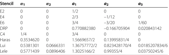
where the grid functions areuj=u(xj) for ≤j≤N, the derivatives are denoted by a prime,u_j,his the space step, andαkandakare given coefficients. IfNc=  the scheme is termed explicit, while compact schemes (also known as implicit or Padé schemes), by con-trast, haveNc=  and require the solution of a matrix equation to determine the deriva-tives along a grid line. Conventionally, the coefficientsαkandakare chosen to provide the largest possible exponent,n, in the truncation error, for a given stencil width, but in some instances some of these coefficients are determined to provide improved dispersion char-acteristics of the scheme. Table  includes some of these weights for various explicit and compact finite difference schemes: the explicit classical second order scheme (E), the ex-plicit classical fourth order scheme (E), the exex-plicit classical sixth order scheme (E), the dispersion-relation-preserving scheme of Tam and Webb [], the compact classical fourth order scheme (C), the optimized tridiagonal compact scheme of Haras and Ta’asan [] (Haras), the optimized pentadiagonal scheme of Lui and Lele [] (Lui), and the spectral-like pentadiagonal compact scheme of Lele [] (Lele). The prefactored compact scheme of Hixon [, ] is also included here in the form

auF_j+ +cuF_j– + ( –a–c)uF_j= h

buj+– (b– )uj– ( –b)uj–

,

cuB_j+ +auB_j– + ( –a–c)uB_j= h

( –b)uj+– (b– )uj–buj–

,

()

whereF andBstand for ‘forward’ and ‘backward’, respectively (in a predictor-corrector time marching framework). For sixth order accuracy,a= / – /(√),b=  – /(a), andc= . The leading order term in the truncation error of a finite difference scheme depends on the choice of the coefficients and the (n+ )st derivative of the functionu.

To study the wave number characteristics of finite difference schemes, consider a pe-riodic domain in real space,x∈[,L], withNuniformly spaced points (the spatial step size ish=L/N). The discrete Fourier transform ofuis given asuˆm=_N Nj=uje–ikmxj with m= –N/, . . . ,N/ – , where the wave number iskm= πm/L. Themth component of the discrete Fourier transform ofudenoteduˆ_mis simplyikmuˆm. Taking the discrete Fourier

Table 1 Weights of the selected spatial finite difference stencils

Stencil α1 α2 a1 a2 a3

E2 0 0 1/2 0 0

E4 0 0 2/3 –1/12 0

E6 0 0 3/4 –3/20 1/60

DRP 0 0 0.770882380 –0.166705904 0.020843142

C4 1/4 0 3/4 0 0

Haras 0.3534620 0 1.5669657/2 0.13995831/4 0

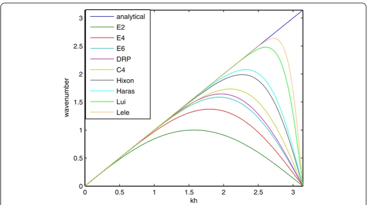
Figure 1 Numerical wave number compared to the analytical wave number.

transform of () implies that

ˆ

u_mnum=iK(kmh)uˆm, ()

where the numerical wave number is given as

K(z) = Ne

n=ansin(nz)  + Nc

n=αncos(nz)

. ()

Figure  shows the numerical wave number for various explicit and compact schemes, corresponding to those given in Table . The numerical wave number is compared to the analytical wave number which is represented by the straight line in Figure . As one can no-tice, the compact schemes are superior to the explicit schemes; however, compact schemes are computationally more demanding because large matrices have to be inverted.

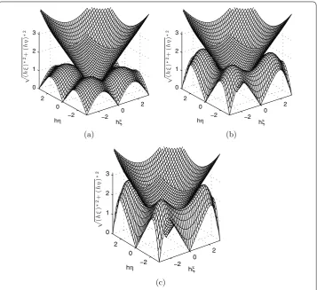
In the multi-dimensional case, the numerical wave number and the numerical phase and group velocity are also dependent on the direction of propagation. Figure  shows the nu-merical wave number surface for the wave equation in two dimensions, corresponding to schemes E, E and Hixon as given in Table  and (), respectively. The cone represents the exact wave number surface, obtained by revolving the straight line from Figure  around the vertical axis. One can clearly notice the anisotropy in the numerical wave number surfaces associated with the finite differencing.

A simple way to reveal the numerical anisotropy is by considering the advection equa-tion in two dimensions,

∂tu= c∇u, ()

with the initial conditionu(r, ) =u(r), where r = (x,y) is the vector of spatial coordinates,

c=c(cosαsinα) is the velocity vector (cis a scalar andαthe propagation direction angle),

Figure 2 Numerical wave number surfaces compared to the analytical wave number surface. (a)Second order explicit scheme (E2);(b)sixth order explicit scheme (E6);(c)sixth order prefactored compact scheme (Hixon). The cones represent the exact wave number surfaces.

on a square grid is obtained as

dtu= – c h

cosα(ui+,j–ui–,j) +sinα(ui,j+–ui,j–)

, ()

wherehis the grid step. Consider the Fourier-Laplace transform:

˜

u(ξ,η,ω) =  (π)

∞



∞

–∞u(x,y,t)e

–i(ξx+ηy–ωt)_{dx dy dt, ()}

whereξ=Kcosαandη=Ksinαare the components of the wave number andωis the fre-quency (Kis the wave number magnitude). The application of Fourier-Laplace transform to () gives the exact dispersion relation:

ω=cKcosα+sinα=cK. ()

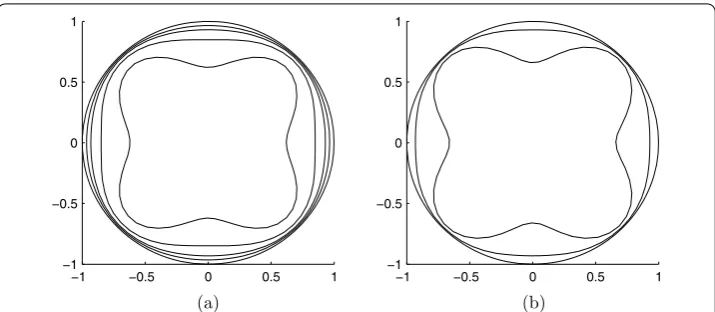
Figure 3 Polar diagram of normalized phase velocities as a function of points per wavelength (PPW) and the direction of propagation. (a)Fourth-order explicit schemes (lowest number of points per wavelength is 4);(b)sixth-order compact schemes (lowest number of points per wavelength is 3).

the same phase velocity in all directions (it is isotropic). Moreover, the exact group velocity defined asge=∂ω/∂K=cis the same as the exact phase velocity because the dispersion relation is a linear function ofK.

We now apply the same Fourier-Laplace transform to the numerical approximation () and obtain the numerical dispersion relation in the form

ω= c h

cosαsin(Khcosα) +sinαsin(Khcosα). ()

The numerical phase velocity will be given as

cn=

ω

K = c Kh

cosαsin(Khcosα) +sinαsin(Khcosα). ()

The constant phase lines are expressed by the equationxcosα+ysinα–cnt= const and move with the phase velocitycn. The numerical anisotropy is revealed in () by the dependence of the numerical phase velocity on the propagation direction angleα. In ad-dition, the numerical group velocity is different from the numerical phase velocity (while previously, in the continuous case, they were the same),

gn=∂Kω=c

cosαcos(Khcosα) +sinαcos(Khsinα), ()

which is also dependent on the propagation direction. This directional dependence of both phase and group velocities defines the numerical anisotropy. As an illustration, Figure  shows polar diagrams for two typical schemes, the fourth order explicit E and the sixth order compact C schemes, revealing the numerical anisotropy (the circle of radius  in Figure  represents the exact solution).

3 Reduction of the numerical anisotropy

3.1 Wave equation

Although the behavior of the numerical anisotropy was often reported in various one-dimensional optimizations of finite difference schemes, one of the first systematic at-tempts to specifically reduce the numerical anisotropy in finite difference schemes was introduced by Trefethen [] in the framework of wave equation. To illustrate Trefethen’s approach, let us consider the two-dimensional wave equation in the form

∂ttu=∂xxu+∂yyu, ()

defined in R _{× [,∞), with appropriate initial and boundary conditions. Using the}

Fourier-Laplace transform, it is ease to find the exact dispersion relation in the form

ω_=ξ_+η_{, where ωis the frequency and (ξ,η) is the wave number vector. Equation}

() was discretized by Trefethen [] on a Cartesian grid, using second order accurate schemes for both temporal and spatial derivatives as

un_ij+–un_ij+un_ij–=k



h

un_i+,j+un_i–,j+un_i,j++un_i,j–– un_i,j ()

which was labeledLF_{. Then the same scheme was used to discretize (), except the}

spatial derivatives were approximated along the diagonal directions with the space step

√

h; the latter discretization was termedLF_{. It was found that the weighted averaging}

/LF_{+ /LF}

provided a low numerical anisotropy in the order of (

ξ_+η_h)_{. Slightly}

the same approach was used by Vichnevetsky [] who corrected the numerical isotropy of the wave propagation in two dimensions using either the linear advection equation or the wave equation.

In a series of papers, Sescuet al.[–] proposed a technique to derive explicit multi-dimensional finite difference schemes for wave equation and Euler equations. By using the transformation matrix between two orthogonal reference frames, one aligned with the grid line and the other along the diagonal direction, the multi-dimensional finite difference scheme was obtained as

where the multi-dimensional space shift operator Eν

x·ui,j=ui+ν,j(see Vichnevetsky and Bowles [] for one dimension) is used. The coefficientsanare those from the classical centered explicit schemes. The operator Dν

x·was defined as Dνx·= (EνxEyν+ E–xνEνy)·The pa-rameterβis called isotropy corrector factor (ICF). The application of the Fourier trans-form to the multi-dimensional schemes gives the numerical wave number

(ξh)∗_opt= 

Then the numerical dispersion relation corresponding to two-dimensional wave equa-tion was considered in the formω– [(ξh)∗

opt+ (ηh)∗opt] = , and the ICF was determined

the xand thex=ydirections. Two curves in wave number-frequency space were con-sidered: one was the intersection between the numerical dispersion relation surface and

η=  plane, and the other was the intersection between the numerical dispersion relation

surface and theξ=ηplane. These two curves were superposed in the (Kh,ω) plane, where Kh= [(ξh)_{+ (ηh)}_]_{. Assuming that the equations of the two curves in (Kh,ω) plane are}

ω=ω(Kh,β) andω=ω(Kh,β), the integrated error between the phase velocities was

then calculated on a specified interval asC(β) =_η|c(Kh,β) –c(Kh,β)|d(Kh), where

c(Kh,β) andc(Kh,β) are the numerical phase velocities. The minimization was done by

equating the first derivative ofC(β) orG(β) with zero, which provided the value of ICF,β. Sescuet al.[, ] conducted a comprehensive stability analysis of the multi-dimen-sional schemes combined with either linear-multistep or multistage time marching schemes, and obtained several noteworthy results. For the Leap-Frog scheme applied to the advection equations, it was shown that the stability restriction corresponding to multi-dimensional schemes differs from the corresponding stability restriction via conventional schemes by the factor (β+ )/(β+ ), whereβis the isotropy corrector factor. The con-clusion was that the stability restrictions corresponding to multi-dimensional schemes are more convenient compared to the conventional schemes. For an arbitrary direction of the convection velocity with|cx| ≥ |cy|, the stability restriction for conventional stencils was given byσx+σy≤CFL, whereσx=k|cx|/handσy=k|cy|/h. For multi-dimensional stencils the stability restriction was given by ( +β)σx+σy≤CFL( +β) (where, for ex-ample,CFLis , . or . corresponding to E, E or E scheme, respectively). Adams-Bashforth and Runge-Kutta time marching schemes in combination with con-ventional and multi-dimensional schemes were also analyzed, and it was found that the multi-dimensional schemes provide less restrictive stability limits.

3.2 Helmholtz equation

Tam and Webb [] performed an anisotropy correction of the finite difference represen-tation of the Helmholtz equation,

∇_p+ξ_{p=f, ()}

wherepis the pressure perturbation,∇_{is the Laplacian operator,f is the source}

distribu-tion (e.g., a monopole),ξ= π/λis the wave number, andλis the acoustic wavelength. Tam and Webb [] showed that the finite difference discretization of the Helmholtz equation,

pi+,j– pi,j+pi–,j

h +

pi,j+– pi,j+pi,j–

h +ξ

_p

i,j=fi,j ()

with five grid points per wavelength introduces significant numerical anisotropy (equally spaced grid is assumed in both thex- andy-direction, and the spatial step is denoted as before byh). They constructed an anisotropy correction factor using asymptotic solutions to the continuous equation () and its finite difference approximation () as

pa(r,θ)rij→∞=

π ξ

π

ir/e

i(ξr–π/)_F¯_α¯

s,β¯+(α¯s)

and

pn(rij,θij)rij→∞=

eiKijrij

r/_ij

G

θij+

G(θij rij

+Or–/_ij , ()

respectively, where (rij,θij) are polar coordinates,Kij=αs(θij)cosθij+βs(θij)sinθij(withαs andβsbeing the wave number components from the Fourier transform), andG(θij) and G(θij) are functions depending onαs,βs,θ, and the Fourier transformF¯of the source term (for more details see () and () in Tam and Webb []). The anisotropy corrector factor was then defined by the ratio between the absolute values of the two,

D(θ,ξh) =|pa|

|pn|

. ()

The correction factor is independent of the distribution of sources, meaning that it can be computed once and for all types of sources. A significant reduction of the anisotropy error was obtained.

3.3 Advection equation

Gaitonde and Shang [] proposed a class of high-order compact difference-based finite-volume schemes which minimized the dispersion and isotropy error functions for the range of wave numbers of interest. The starting point was the one-dimensional advection equation,

∂tu+∂xf = , f =cu,c>  ()

which was discretized using a finite volume approach as

dtu¯i+f¯i+/–¯fi–/= , ()

whereu¯is the average value ofuinside a cell,u¯= /hxi+/

xi–/ u dx, andf¯is the flux function

approximatingf, which is dependent on the values ofu¯from neighbor cells. The recon-struction can be done by considering a primitive functionv=_xwhich must be discretized at the cell interface. Gaitonde and Shang [] considered a five-point compact stencil in the form

αvi–/+vi+/+αvi+/=b

vi+/–vi–/

h +a

vi+/–vi–/

h , ()

where α,a, andb are constants which determine the order of accuracy of the scheme. Using Taylor series expansions, they sacrificed the order of accuracy of the schemes by writingaandbas functions ofα,

a=( +α)

 , b=

– + α

 ()

The spectral function associated with the scheme () is given as

ˆ

A(w) =i(asin(w) +bsin(w)/)

wherew= π ξh/Lis the scaled wave number. The dispersion error is associated with the

whereθ is the angle that the direction of propagation makes with the x-axis. An isotropy error function was defined by Gaitonde and Shang [] in the form

Ei(α,wmax) =

which was minimized to find the value ofαoptthat gives the lowest numerical anisotropy.

Numerical examples confirmed a considerable reduction of the isotropy error.

Sescu and Hixon [, ] extended the previous optimization performed in [] to prefactored compact finite difference schemes [, ] applied to the advection equation. The prefactored compact schemes are defined on a three-point stencil and can return up to eight orders of accuracy (see equations ()). They can be used within a predictor-corrector type time marching scheme framework (MacCormack []), because the nu-merical derivatives are determined by sweeping from one boundary to the other, in both directions. Following the same analysis as in the case of explicit schemes, the multi-dimensional prefactored compact schemes were obtained as

uF_i,j= α

for fourth order of accuracy, and

for sixth order of accuracy.βis the isotropy corrector factor (ICF) and its magnitude can be determined by minimizing the dispersion error corresponding to the wave-front prop-agating along a grid line and the wave-front propprop-agating along a diagonal direction.

Using Fourier analysis, the numerical wave numbers and the numerical dispersion re-lation corresponding to the two-dimensional wave equation were found. The individual (forward or backward) numerical wave number has both real and imaginary parts: the real part of the forward operator is equal to the real part of the backward operator, and the imaginary parts are opposite. As a result, in a MacCormack predictor-corrector scheme the overall imaginary part is zero. The real parts of the numerical wave numbers corre-sponding to multi-dimensional schemes, for derivatives along thex-direction, were given by

In terms of numerical stability, more efficient stability restrictions were obtained as in the case of multi-dimensional explicit schemes. For example, multi-dimensional MacCor-mack schemes were found to provide a stability restriction in the form

it goes to /(ξmax)/whenβ→ ∞. This generated more efficient stability restrictions by

using multi-dimensional compact schemes. Test cases showed that the multi-dimensional compact schemes were more efficient for both the fourth and the sixth order accurate schemes.

3.4 Maxwell equations

Sun and Trueman [] performed an optimization of finite difference schemes applied to the Maxwell equations, in terms of reducing the dispersion and isotropy errors. For brevity, we show here the numerical dispersion relations (for finite differencing represen-tations of the Maxwell equations, see (), (), and () in Sun and Trueman []):

corresponding to a grid line, and

corresponding to the diagonal direction, wherewis a weighting factor,βais the numerical phase constant along the grid line,βdis the numerical phase constant along the diagonal direction,ωis the frequency, andkis the time step (an equally spaced grid is considered again). The optimization in terms of reducing the numerical anisotropy was done by elim-inating the time step terms in () and () to obtain

wi=

This optimal weightwiis a function of mesh density only, and is not dependent on the time step size or the frequency of the signal. This method theoretically provides a uniform phase velocity in all directions. Further optimizations of this scheme were performed in another paper of Sun and Trueman [].

Kohet al.[] derived a two-dimensional finite-difference time-domain method, dis-cretizing the Maxwell equations, to eliminate the numerical dispersion and anisotropy. The proposed scheme is given as

d_tH_xn_,i,j+/= – k

t is the central difference operator with respect to time,

dpfq=

wheref is a generic function. In (),Eis the electric field,His the magnetic field strength,

σ,μ, andare the conductivity, the permeability, and the permittivity, respectively, of the domain,kis the time step, andhis the spatial step in all directions. For nonconductive media,σ= , the numerical dispersion relation can be obtained as



is given as

An optimal value forα, achieving an isotropic numerical phase velocity, can be simply estimated as the mean value ofαover the azimuthal angles, and it was found that it remains constant (approximately, .) for a wide range of grid sizes, and it is insensitive to the value of the Courant number.

Kim et al. [] derived new three-dimensional isotropic dispersion-finite-difference time-domain schemes (ID-FDTD) based on a linear combination of the traditional cen-tral difference equation and a new difference equation based on the extra sampling points. They used the same scaling factors as for the two-dimensional case to attain the isotropic dispersion and the exact phase velocity. Based on the weighting factors, seven different FDTD schemes were formulated, including the Yee scheme []. Among the seven pro-posed FDTD schemes, three showed improved isotropy of the dispersion compared to the dispersion of the Yee scheme. For the sake of brevity, the complete expressions of the schemes are not included here (see Kim et al.[] for more details), and only the nu-merical dispersion relation is briefly presented. Plane wave solutions were introduced in discretized forms as

En_i,j= EeI(nωk–ξih–ηjh–ζkh), ()

Hn_i,j= HeI(nωk–ξih–ηjh–ζkh), ()

whereI=√–,ωis the frequency, (ξ,η,ζ) is the numerical wave number vector, and E

and Hare constant vectors. After inserting () and () into the discretized form of

the Maxwell equations (see () in Kimet al.[]), the matrix equations are obtained as CH=StE,CE=SiμHwhere

and the numerical dispersion relation was obtained by vanishing of the associated deter-minant,

et al.[] used the scaling factor from the two-dimensional case, and they modified the numerical dispersion relation to estimate the weighting factors.

3.5 Dendritic solidification

Kumar [] derived isotropic finite difference schemes for the first and second derivatives in the context of symmetric dendritic solidification. The first derivative was discretized as

(∂xu)I,i,j=  h



(ui+,j+–ui–,j+) + 

(ui+,j–ui–,j) + 

(ui+,j––ui–,j–)

, ()

which involves grid points not only along thex-direction, but also along they-direction. The Taylor expansion of the scheme () can be written as (∂xu)I,i,j= ( +h/∇)(∂xu)i,j, where the leading order term involves the Laplacian only, implying no directional depen-dence. The second derivative was discretized as

(∂xxu)I,i,j=  h



(ui+,j+– ui,j+ui–,j+) + 

(ui+,j– ui,j+ui–,j)

+ 

(ui+,j–– ui,j–+ui–,j–)

, ()

where the Taylor expansion is given by (∂xxu)I,i,j= ( +h/∇)(∂xxu)i,j, it being again a function of the Laplacian only. The conventional cross derivative (∂xyu)I,i,jwas found to be intrinsically isotropic according to the criterion developed by Kumar []. The Lapla-cian can be obtained by combining the isotropic derivatives along the x- and y-directions, (∇_u)

i,j= (∂xxu)I,i,j+ (∂yyu)I,i,j. A significant reduction of the numerical anisotropy was ob-tained by using these schemes. Shen and Cangellaris [] exploited further this approach to develop new isotropic finite-difference time-domain schemes modeling electromag-netic wave propagation.

4 Concluding remarks

Future directions should focus on optimizations of existing compact finite difference schemes in terms of reducing the numerical anisotropy, or derivations of novel com-pact schemes with low numerical anisotropy. Optimizations and derivations of finite vol-ume schemes (in terms of reducing the nvol-umerical anisotropy) applied to either struc-tured or unstrucstruc-tured grids should also be taken into account, especially in the framework of wave propagation problems. Filtering schemes, as applied, for example, in large eddy simulations to separate the small scales from the large scales, may experience numerical anisotropy since they are effective at high wave number ranges. Optimizations of such fil-ters in terms of reducing the numerical anisotropy is also another future area of research.

Competing interests

The author declares that they have no competing interests.

Acknowledgements

The author would like to thank Ray Hixon, Abdollah Afjeh, Vasanth Allampalli, Shivaji Medida, Daniel Ingraham, and Carmen Sescu for constructive support and encouragement.

Received: 15 July 2014 Accepted: 25 December 2014

References

1. Lele, SK: Compact finite difference schemes with spectral-like resolution. J. Comput. Phys.103, 16-42 (1992) 2. Tam, CKW, Webb, JC: Dispersion-relation-preserving finite difference schemes for computational aeroacoustics.

J. Comput. Phys.107, 262-281 (1993)

3. Kim, JW, Lee, DJ: Optimized compact finite difference schemes with maximum resolution. AIAA J.34, 887-893 (1996) 4. Zingg, DW, Lomax, H, Jurgens, HM: High-accuracy finite-difference schemes for linear wave propagation. SIAM J. Sci.

Comput.17, 328-346 (1996)

5. Mahesh, K: A family of high order finite difference schemes with good spectral resolution. J. Comput. Phys.145, 332-358 (1998)

6. Hixon, R: Prefactored small-stencil compact schemes. J. Comput. Phys.165, 522-541 (2000) 7. Ashcroft, G, Zhang, X: Optimized prefactored compact schemes. J. Comput. Phys.190, 459-477 (2003) 8. Fauconnier, D, De Langhie, C, Dick, E: A family of dynamic finite difference schemes for large-eddy simulation.

J. Comput. Phys.228, 1830-1861 (2009)

9. Laizet, S, Lamballais, E: High-order compact schemes for incompressible flows: a simple and efficient method with quasi-spectral accuracy. J. Comput. Phys.228, 5989-6015 (2009)

10. Hu, FQ, Hussaini, MY, Manthey, JL: Low-dissipation and low-dispersion Runge-Kutta schemes for computational acoustics. J. Comp. Physiol.124, 177-191 (1996)

11. Stanescu, D, Habashi, WG: 2N-storage low-dissipation dispersion Runge-Kutta schemes for computational acoustics. J. Comput. Phys.143, 674-681 (1998)

12. Mead, JL, Renaut, RA: Optimal Runge-Kutta methods for first order pseudospectral operators. J. Comp. Physiol.152, 404-419 (1999)

13. Bogey, C, Bailly, C: A family of low dispersive and low dissipative explicit schemes for flow and noise computation. J. Comp. Physiol.194, 194-214 (2004)

14. Berland, J, Bogey, C, Bailly, C: Low-dissipation and low-dispersion fourth-order Runge-Kutta algorithm. Comput. Fluids35, 1459-1463 (2006)

15. Vichnevetsky, R, Bowles, JB: Fourier Analysis of Numerical Approximations of Hyperbolic Equations. SIAM Studies in Applied Mathematics. SIAM, Philadelphia (1982)

16. Trefethen, LN: Group velocity in finite difference schemes. SIAM Rev.24, 113 (1982)

17. Zingg, DW, Lomax, H: Finite difference schemes on regular triangular grids. J. Comput. Phys.108, 306-313 (1993) 18. Tam, CKW, Webb, JC: Radiation boundary condition and anisotropy correction for finite difference solutions of the

Helmholtz equation. J. Comput. Phys.113, 122-133 (1994)

19. Jo, CH, Shin, CS, Suh, JH: An optimal 9 point finite difference, frequency-space, 2-D wave extrapolator. Geophysics61, 529-537 (1996)

20. Hustesdt, B, Operto, S, Virieux, J: Mixed-grid and staggered-grid finite-difference methods for frequency-domain acoustic modeling. Geophys. J. Int.157, 1269-1296 (2004)

21. Lin, RK, Sheu, TWH: Application of dispersion-relation-preserving theory to develop a two-dimensional convection-diffusion scheme. J. Comput. Phys.208, 493-526 (2005)

22. Kumar, A: Isotropic finite-differences. J. Comput. Phys.201, 109-118 (2004)

23. Patra, M, Karttunen, M: Stencils with isotropic discretization error for differential operators. Numer. Methods Partial Differ. Equ.22, 936-953 (2006). doi:10.1002/num.20129

24. Stegeman, PC, Young, ME, Soria, J, Ooi, A: Analysis of the anisotropy of group velocity error due to spatial finite difference schemes from the solution of the 2D linear Euler equations. Int. J. Numer. Methods Fluids71, 805-829 (2013)

25. Sescu, A, Hixon, R, Afjeh, AA: Anisotropy Correction of Two Dimensional Finite Difference Schemes for Computational Aeroacoustics. AIAA Paper 2007-3495 (2007)

27. Sescu, A, Afjeh, AA, Hixon, R: Optimized difference schemes for multidimensional hyperbolic PDEs. Electron. J. Differ. Equ. Conf.17, 213-225 (2009)

28. Sescu, A, Hixon, R, Sescu, C, Abdollah, AA: Stability Investigation of Multidimensional Optimized Spatial Stencils. AIAA Paper 2009-0005 (2009)

29. Sescu, A, Hixon, R: Multidimensional Prefactored Compact Schemes. AIAA Paper 2012-1175 (2012) 30. Sescu, A, Hixon, R: Numerical anisotropy study of a class of compact schemes. J. Sci. Comput. (2014).

doi:10.1007/s10915-014-9826-0

31. Berini, J, Wu, K: A comprehensive study of numerical anisotropy and dispersion in 3-D TLM meshes. IEEE Trans. Microw. Theory Tech.43, 1173-1181 (1995)

32. Gaitonde, D, Shang, JS: Optimized compact-difference-based finite-volume schemes for linear wave phenomena. J. Comput. Phys.138, 617-643 (1997)

33. Sun, G, Trueman, CW: Optimized finite-difference time-domain methods based on the (2, 4) stencil. IEEE Trans. Antennas Propag.53, 832-842 (2005)

34. Sun, G, Trueman, CW: Suppression of numerical anisotropy and dispersion with optimized finite-difference time-domain methods. IEEE Trans. Antennas Propag.53, 4121-4128 (2005)

35. Koh, I, Kim, H, Lee, J-M, Yook, J-G, Pil, CS: Novel explicit 2-D FDTD scheme with isotropic dispersion and enhanced stability. IEEE Trans. Antennas Propag.54, 3505-3510 (2006)

36. Shen, G, Cangellaris, AC: A new FDTD stencil for reduced numerical anisotropy in the computer modeling of wave phenomena. Int. J. RF Microw. Comput.-Aided Eng.17, 447-454 (2007)

37. Kim, W-T, Koh, I-S, Yook, J-G: 3D isotropic dispersion (ID)-FDTD algorithm: update equation and characteristics analysis. IEEE Trans. Antennas Propag.58, 1251-1259 (2010)

38. Yee, K: Numerical solution of initial boundary value problems involving Maxwell’s equations in isotropic media. IEEE Trans. Antennas Propag.14, 302-307 (1966)

39. Kong, Y-D, Chu, Q-X: An unconditionally-stable FDTD method with low anisotropy in three-dimensional domains. In: Proceedings of Progress in Electromagnetics Research Symposium, Kuala Lumpur, Malaysia (2012)

40. Haras, Z, Ta’asan, S: Finite-difference schemes for long-time integration. J. Comput. Phys.114, 265-279 (1994) 41. Lui, C, Lele, SK: Direct Numerical Simulation of Spatially Developing, Compressible, Turbulent Mixing Layers. AIAA

Paper 2001-0291 (2001)

42. Hixon, R, Turkel, E: Compact implicit MacCormack-type schemes with high accuracy. J. Comput. Phys.158, 51-70 (2000)

43. Sescu, A, Afjeh, AA, Hixon, R, Sescu, C: Conditionally stable multidimensional schemes for advective equations. J. Sci. Comput.42, 96-117 (2009)