R E S E A R C H
Open Access
The application of block pulse functions
for solving higher-order differential equations
with multi-point boundary conditions
Zakieh Avazzadeh
1*and Mohammad Heydari
2*Correspondence: [email protected] 1Institute of Mathematics, School of Mathematical Sciences, Nanjing Normal University, Nanjing, 210023, China
Full list of author information is available at the end of the article
Abstract
In this paper, the block pulse function method is proposed for solving high-order differential equations associated with multi-point boundary conditions. Although the orthogonal block pulse functions frequently have been applied to approximate the solution of ordinary differential equations associated with the initial conditions, the presented method provides the flexibility with respect to multi-point boundary conditions in separated or non-separated forms. This technique, which may be named the augmented block pulse function method, reduces a system of high-order boundary value problems of ordinary differential equations to a system of algebraic equations. The illustrated results confirm the computational efficiency, reliability, and simplicity of the presented method.
MSC: 65Lxx; 94A11; 34k28
Keywords: ordinary differential equations; block pulse functions; boundary value problem; multi-point value problem; separated or non-separated boundary conditions
1 Introduction
The systems of ordinary differential equations (ODEs) with different boundary conditions are well known for their applications in biology, chemistry, physics, engineering, and sci-ences [–]. There are many different reliable methods which can find the solution of ODEs for simple forms of boundary conditions. But the mathematical models of many phenomena in the real world are enforced by more difficult forms of boundary conditions such as multi-point boundary conditions in separated or non-separated forms.
Because of the importance, the boundary value problems have been solved several times by many different methods such as the finite difference method, the spline method, the ra-dial basis functions, the wavelet method, and many other numerical and analytical meth-ods; see [–] and the references therein. We recall that boundary conditions that are more difficult imply developing numerical methods to find the solution of the ordinary differential systems. However, some of these methods are reliable and applicable for solv-ing ordinary differential equations; the most of these methods provide the solution only for a particular kind of differential equations or a particular kind of boundary conditions.
In this study, we describe the application of the block pulse function method for solving arbitrary-order differential equations.
Recently, orthogonal block pulse functions have been widely discussed and applied to approximate the solutions of some difficult systems defined in engineering and science [–]. The most important properties of BPFs are disjointness, orthogonality, and com-pleteness which cause the popularity among the computational methods.
In this work, we proposed the augmented block pulse function method for solving a system of arbitrary-order boundary value problem associated with initial conditions or multi-point boundary conditions in separated or non-separated forms. Let us consider the followingnth-order differential equations with assumption of the existence and unique-ness of the solution:
LF(x),x= , x∈[a,b], ()
associated withnequality conditions and
F(x) =f(n)(x),f(n–)(x), . . . ,f(x),f(x). ()
Since the differential equation may be enforced by many different conditions, we consider the general form including separated and non-separated boundary conditions but we also can consider boundary conditions or the set of conditions including some or all of these mentioned types. Let us assume
Lf(x),f(x), . . . ,f(xk)
= ,
Lf(x),f(x), . . . ,f(xk)= , ..
.
Lnf(x),f(x), . . . ,f(xk)= ,
()
andx∈Randx,x, . . . ,xk(not necessarily distinct) are given real finite constants. Ifk= the problem becomes the initial value problem and fork= the problem will be called a two-point boundary value problem. It is also called a multi-point boundary value prob-lem ifk> . In the particular case of distinctx,x, . . . ,xn, the boundary conditions of the
following type:
Lf(x)= ,
Lf(x)= , ..
.
Lnf(xn)= ,
derivatives off(x) so
LF(x),F(x), . . . ,F(xk)
= ,
LF(x),F(x), . . . ,F(xk)
= ,
.. .
LnF(x),F(x), . . . ,F(xk)
= .
()
However, these types of systems arising in engineering and sciences have important ap-plications but it is not possible to solve them analytically for arbitrary choices ofL(x) and
Li(x),i= , , . . . ,n. Therefore, the numerical methods for obtaining an approximated so-lution of () with higher accuracy still is of interest for researchers.
To make the article self-contained in Section a short description on block pulse func-tions is added. In Section the description of the method shows BPFs how can be applied to solve the high-order differential equations with a different kind of boundary conditions. The numerical results are illustrated in Section to clarify more details of the proposed method and expectedly confirm the convergence and applicability of the method. Finally, a brief conclusion is stated in Section .
2 Block pulse functions
Anm-set of BPFs over the intervalt∈[, ) is defined as follows []:
βi(x) = ⎧ ⎨ ⎩
, x∈[mi,i+m), , otherwise,
()
wherei= , , . . . ,m– is the translation parameter andβi(x) is called theith BPF.
There are some properties for BPFs which make them popular for approximation such as orthogonality, disjointness, and completeness []. A function f(x) over the interval [, ), can be expanded in a BPFs series with an infinite number of terms
f(x) =
∞
i=
ciβi(x), x∈[, ), ()
where the coefficients are calculated as follows:
ci=m
f(x)βi(x)dx, i= , , . . . . ()
In fact, the series expansion () contains an infinite number of terms for smoothf(x). If
f(x) is a piecewise constant or may be approximated by a piecewise constant, the sum in () will be terminated aftermterms, that is,
f(x)
m–
i=
ciβi(x) = CTmm(x), x∈[, ), ()
where
Cm= [c,c, . . . ,cm–]T and m(x) = β(x),β(x), . . . ,βm–(x) T
Also, the collocation points can be defined in the following form:
ξl=
l–
m , l= , , . . . ,m, ()
Now substituting the collocation points leads to
f(ξl) m–
i=
ciβi(ξl) = CTmm(ξl), l= , , . . . ,m. ()
The above equations can be rewritten in the following matrix form:
FT= CTmm, where F = f(ξ),f(ξ), . . . ,f(ξm–) T
, ()
andmis the BPF matrix of ordermdefined by
m= Im=diag(, , . . . , ). ()
Theorem .[, ] Suppose that f(x)is an arbitrary real bounded function,which is square integrable in the interval[, ),and
em(x) =f(x) –
We consider the solution ofnth-order system () to need at leastnth-order differentia-bility to be able to approximate the highest-order derivative of the unknown function and prevent the discontinuity seen in (). So we first define
These integrals can be evaluated using the definition of BPFs fori= , , . . . ,m– and are
Remark . More generally, we define the BPFs over the interval [a,b) as
¯
Note that if we assume
f(n)(x)
Similarly, by using the collocations points () we have
f(ξl)
and the matrix form of the above linear system is
where
is thenth BPFs integral matrix and
Tj= ξk,ξk, . . . ,ξmk T
, j= , , . . . ,n– . ()
For example, the matrix of the first time integration is
()m =
and the second time integration is
()m =
The integration of BPFs has the important role to approximate differential terms and the described matrices in (), (), and () show the sparsity of the systems made by using BPFs, which affects the computational efficiency.
3 Description of the method
First we describe the method for general form of () and then some particular cases will be taken to show more features of the method. Assumef(n)(x) is expanded in a series as
f(n–)(x) =
In closed form we can write
f(x) =
This assumption leads to the technique which we named the augmented block pulse function (ABPF) method. In fact, we develop the BPF method to be flexible for an approx-imation of the differential equations with different boundaries. We replace the expansion off(i)(x),i= , , . . . ,n, into the system of () and () and then substitute the collocation points defined in () as follows:
LF(ξl),ξl
and
LF(x),F(x), . . . ,F(xk)= ,
LF(x),F(x), . . . ,F(xk)= , ..
.
LnF(x),F(x), . . . ,F(xk)= ,
()
where
F(ξl) =
f(n)(ξl),f(n–)(ξl), . . . ,f(ξl),f(ξl)
, l= , , . . . ,m. ()
From equations () and (), a nonlinear system of (m+n) equations and (m+n) unknown coefficients results. Solving this system, we can obtain the unknown coefficients ci,i= , , . . . , (m+n– ) and therefore the functionsf(j)(x),j= , , . . . ,nare identified.
Remark . It is worth noting here that we can do a few simple modifications when some
off(i)(a),i= , , . . . ,n– , are given. Particularly iff(i)(a),i= , , . . . ,n– , all are given,
the system becomes an initial value problem and there is no need to consider anyci,i=
m, . . . ,m+n– . In addition, we can keep the structure of the algorithm and input the given initial value into the described scheme. Obviously, the first state considers the value off(i)(a),i= , , . . . ,n– , precisely and the second state find them approximately such
that there are good agreement between precise and approximated values. In this paper, the reported results are based on the second assumption.
Remark . Definitely we need (n+m) equations which are linear independent to find
a unique solution including (n+m) unknown coefficients. Note that the intersection of
{x,x, . . . ,xk}defined in (), and the collocation points defined () should be an empty set. If there exists any common point, we can simply change the collocation points non-uniformly such that every collocation point may be chosen from [i
m, i+
m),i= , , , . . . , m– in order to include all basis functions and keep the structure of constructed matrices demonstrated in (), (), and () and for higher order. Obviously, there are many sets of points that are appropriate candidates for leading to the independent algebraic equations.
4 Numerical examples
In order to assess the accuracy of block pulse function method for solving higher-order differential equations with multi-point boundary conditions we will consider the follow-ing examples. The associated computations with the examples were performed usfollow-ing MAPLE with digits precision on a personal computer.
Example Consider the following ordinary differential equation [, ]:
with the separated boundary conditions
and the exact solution
y(x) =x– sin(x).
According to the algorithm, we first approximatey()(x) as follows:
y()(x) into the following equation:
Table 1 The observed maximum absolute error for different values ofmfor Example 1
y(j) m = 6 m = 10 m = 16 m = 32
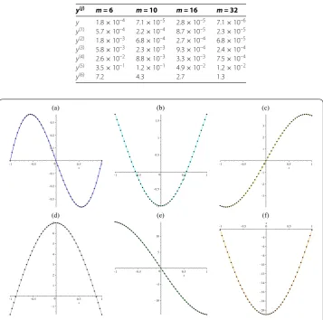
y 1.8×10⁻⁴ 7.1×10⁻⁵ 2.8×10⁻⁵ 7.1×10⁻⁶ y(1) 5.7×10⁻⁴ 2.2×10⁻⁴ 8.7×10⁻⁵ 2.3×10⁻⁵ y(2) 1.8×10⁻³ 6.8×10⁻⁴ 2.7×10⁻⁴ 6.8×10⁻⁵ y(3) 5.8×10⁻³ 2.3×10⁻³ 9.3×10⁻⁴ 2.4×10⁻⁴ y(4) 2.6×10⁻² 8.8×10⁻³ 3.3×10⁻³ 7.5×10⁻⁴ y(5) 3.5×10⁻¹ 1.2×10⁻¹ 4.9×10⁻² 1.2×10⁻² y(6) 7.2 4.3 2.7 1.3
Figure 1 Plots of the numerical solution by BPFs versus the exact solution (solid-circle) ofy,y,y,
y(3),y(4),y(5)in (a)-(f), respectively, whenm= 64 for Example 1.
follows:
i=
ciPi(–) –
c+
c–
c+
c–c+c= ,
i=
ciPi() +
c+
c+
c+
c+c+c= ,
i=
ciPi(–) –
c+
c–c+c+ cos(–) – sin(–) = ,
i=
ciPi() +
c+
c+c+c– cos() + sin() = ,
i=
ciPi(–) –c+c– cos(–) + sin(–) = ,
i=
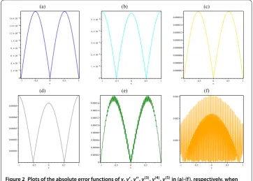
Figure 2 Plots of the absolute error functions ofy,y,y,y(3),y(4),y(5)in (a)-(f), respectively, when
m= 64 for Example 1.
Figure 3 Sixth derivative of the numerical solution by BPFs versus the exact solution whenm= 64 for Example 1.
in which are included unknown coefficients. Solving the obtained system gives
c= –., c= –., c= –.,
c= ., c= ., c= .,
c= –., c= ., c= .,
c= ., c= –., c= .,
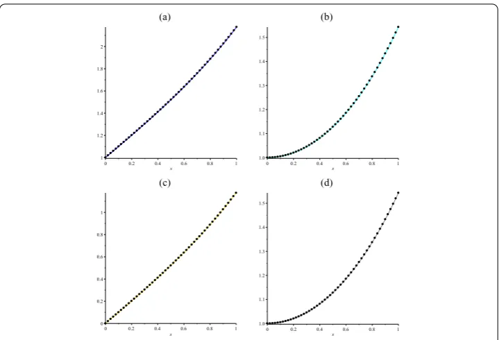
Figure 4 Plots of the numerical solution by BPFs versus the exact solution (solid-circle) ofy,y,y,y(3)
in (a)-(d), respectively, whenm= 64 for Example 2.
solution form= is given in Figure . This example with other boundary conditions [, ] also can be reduced to a system of linear equations as described.
Example Consider the following linear fourth-order nonlocal boundary value problem []:
y()(x) +exy()(x) +y(x) = –excosh(x) + sinh(x), x∈[, ],
with the non-separated boundary conditions
y
= +sinh
, y
=cosh
,
y
=sinh
, y
–y
=sinh
–sinh
,
and the exact solution
y(x) = +sinh(x).
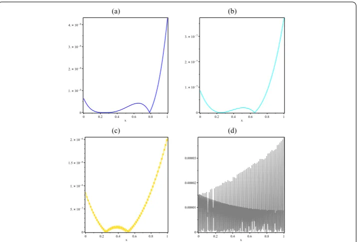
Figure 5 Plots of the absolute error functions ofy,y,y,y(3)in (a)-(d), respectively, whenm= 64 for Example 2.
Figure 6 Fourth derivative of the numerical solution by BPFs versus the exact solution whenm= 64 for Example 2.
Example Consider the following nonlinear second-order four-point boundary value problem:
y(x) –sin(x)y(x) +y(x) = sin(x)
cos(x), x∈[, ],
with the non-separated boundary conditions
y() = , y() –
i=
+i
y
i
= .,
and the exact solution
Table 2 The observed maximum absolute error for different values ofmfor Example 2
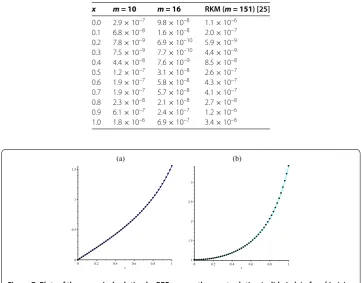
x m = 10 m = 16 RKM (m = 151) [25]
0.0 2.9×10⁻⁷ 9.8×10⁻⁸ 1.1×10⁻⁶ 0.1 6.8×10⁻⁸ 1.6×10⁻⁸ 2.0×10⁻⁷ 0.2 7.8×10⁻⁹ 6.9×10⁻¹⁰ 5.9×10⁻⁹ 0.3 7.5×10⁻⁹ 7.7×10⁻¹⁰ 4.4×10⁻⁹ 0.4 4.4×10⁻⁸ 7.6×10⁻⁹ 8.5×10⁻⁸ 0.5 1.2×10⁻⁷ 3.1×10⁻⁸ 2.6×10⁻⁷ 0.6 1.9×10⁻⁷ 5.8×10⁻⁸ 4.3×10⁻⁷ 0.7 1.9×10⁻⁷ 5.7×10⁻⁸ 4.1×10⁻⁷ 0.8 2.3×10⁻⁸ 2.1×10⁻⁸ 2.7×10⁻⁸ 0.9 6.1×10⁻⁷ 2.4×10⁻⁷ 1.2×10⁻⁶ 1.0 1.8×10⁻⁶ 6.9×10⁻⁷ 3.4×10⁻⁶
Figure 7 Plots of the numerical solution by BPFs versus the exact solution (solid-circle) ofy,yin (a) and (b), respectively, whenm= 32 for Example 3.
Figure 8 Plots of the absolute error functions ofy,yin (a) and (b), respectively, whenm= 32 for Example 3.
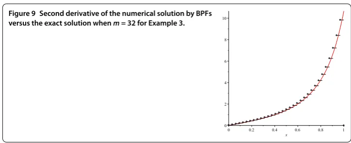
The plots of the numerical solution by the proposed method withm= versus the exact solution and the absolute error function are depicted in Figures and , respectively. The graph of second derivative of the numerical solution by BPFs versus the exact solution for
m= is given in Figure .
5 Conclusion
equa-Figure 9 Second derivative of the numerical solution by BPFs versus the exact solution whenm= 32 for Example 3.
tions by using block pulse functions and a polynomial function of degreen– . The most important privileges of the proposed method are computational efficiency due to sparse matrices, simplicity, and reliability, so one may increase the number of basis functions and consequently the accuracy will be improved.
Competing interests
The authors declare that they have no competing interests.
Authors’ contributions
All authors contributed equally to the writing of this paper. All authors read and approved the final manuscript.
Author details
1Institute of Mathematics, School of Mathematical Sciences, Nanjing Normal University, Nanjing, 210023, China. 2Department of Mathematics, Yazd University, P.O. Box 89195-741, Yazd, Iran.
Acknowledgements
Z Avazzadeh wish to thank Natural Science Foundation of Jiangsu Province (Project No. BK20150964) and gratefully acknowledges ‘A Project Funded by the Priority Academic Program Development of Jiangsu Higher Education Institutions’.
Received: 10 January 2016 Accepted: 30 March 2016 References
1. Agarwal, RP: Boundary Value Problems for High Order Differential Equations. World Scientific, Singapore (1986) 2. Ang, WT, Park, YS: Ordinary Differential Equations: Methods and Applications. Universal-Publishers, Boca Raton (2008) 3. Hsu, S-B: Ordinary Differential Equations with Applications. World Scientific, Singapore (2006)
4. Roberts, C: Ordinary Differential Equations: Applications, Models, and Computing. CRC Press, Boca Raton (2011) 5. Loghmani, GB, Ahmadinia, M: Numerical solution of sixth order boundary value problems with sixth degree B-spline
functions. Appl. Math. Comput.186, 992-999 (2007)
6. Loghmani, GB, Alavizadeh, SR: Numerical solution of fourth-order problems with separated boundary conditions. Appl. Math. Comput.191, 571-581 (2007)
7. Siddiqi, SS, Akram, G: Septic spline solutions of sixth-order boundary value problems. J. Comput. Appl. Math.215, 288-301 (2008)
8. Temimi, H, Ansari, AR: A new iterative technique for solving nonlinear second order multi-point boundary value problems. Appl. Math. Comput.218, 1457-1466 (2011)
9. Vedat, SE: Solving nonlinear fifth-order boundary value problems by differential transformation method. Selçuk J. Appl. Math.8(1), 45-49 (2007)
10. Wazwaz, AM: The numerical solution of fifth-order boundary value problems by the decomposition method. J. Comput. Appl. Math.136, 259-270 (2001)
11. Datta, KB, Mohan, BM: Orthogonal Functions in Systems and Control. World Scientific, Singapore (1995)
12. Deb, A, Sarkar, G, Bhattacharjee, M, Sen, SK: All-integrator approach to linear SISO control system analysis using block pulse functions (BPF). J. Franklin Inst.334(2), 319-335 (1997)
13. Deb, A, Sarkar, G, Sen, SK: Block pulse functions, the most fundamental of all piecewise constant basis functions. Int. J. Syst. Sci.25(2), 351-363 (1994)
14. Harmuth, HF: Transmission of Information by Orthogonal Functions. Springer Science & Business Media. Springer, Berlin (2013)
15. Hatamzadeh-Varmazyar, S, Masouri, Z, Babolian, E: Numerical method for solving arbitrary linear differential equations using a set of orthogonal basis functions and operational matrix. Appl. Math. Model. (2015). doi:10.1016/j.apm.2015.04.048
17. Hatamzadeh-Varmazyar, S, Naser-Moghadasi, M, Masouri, Z: A moment method simulation of electromagnetic scattering from conducting bodies. Prog. Electromagn. Res.81, 99-119 (2008)
18. Hatamzadeh-Varmazyar, S, Naser-Moghadasi, M, Babolian, E, Masouri, Z: Numerical approach to survey the problem of electromagnetic scattering from resistive strips based on using a set of orthogonal basis functions. Prog. Electromagn. Res.81, 393-412 (2008)
19. Jiang, ZH, Schaufelberger, W: Block Pulse Functions and Their Applications in Control Systems. Lecture Notes in Control and Information Sciences, vol. 179. Springer, Berlin (1992)
20. Rao, CP: Piecewise Constant Orthogonal Functions and Their Application to Systems and Control. Springer, Berlin (1983)
21. Sannuti, P: Analysis and synthesis of dynamic systems via block-pulse functions. Proc. Inst. Electr. Eng.124(6), 569-571 (1977)
22. Wang, C-H: Generalized block-pulse operational matrices and their applications to operational calculus. Int. J. Control
36, 67-76 (1982)
23. Maleknejad, K, Khodabin, M, Rostami, M: A numerical method for solvingm-dimensional stochastic Itô-Volterra integral equations by stochastic operational matrix. Comput. Math. Appl.63, 133-143 (2012)
24. Siddiqi, SS, Twizell, EH: Spline solutions of linear sixth order boundary value problems. Int. J. Comput. Math.60, 295-304 (1996)