R E S E A R C H
Open Access
Wireless sensor network localization with
connectivity-based refinement using mass spring
and Kalman filtering
Sangwoo Lee, Hyunjae Woo and Chaewoo Lee
*Abstract
Since many range-free localization algorithms depend on only a few anchors and implicit range estimations, they produce poor results. In this article, we propose a distributed range-free algorithm to improve localization accuracy by using one-hop neighbors as well as anchors. When an unknown node knows which nodes it can directly communicate with, but does not know how far they are exactly placed, the node should have a location having the average distance to all neighbors since the location minimizes the sum of squares of hop distance errors. In the proposed algorithm, each node initializes its location using the information of anchors and updates it based on mass spring method and Kalman filtering with the location estimates of one-hop neighbors until the equilibrium is achieved. Subsequently, the network has the shape of isotropic graph with minimized variance of links between one-hop neighbors. We evaluate our algorithm and compare it with other range-free algorithms through simulations under varying node density, anchor ratio, and node deployment method.
1 Introduction
In wireless sensor networks (WSNs), numerous radio nodes collaborate to allow communication in the absence of a fixed infrastructure. With the flexibility and scalability, WSNs have great potential for a variety of applications including environmental monitoring, health care, target tracking, and military surveillance [1,2]. Most of these applications require the knowledge about the location of each node because data stream of a node presents the state or context in the location. Moreover, the location information is required for some methods such as routing and broadcasting protocols [3] in WSNs with the properties of frequently route breakage and unpredictable topology changes.
Localization/positioning (obtaining the location of a node) has been an essential demand to realize location-based applications and methods in WSNs. GPS [4] may be the most straightforward solution to the localization problem. However, GPS is unavailable in indoor envir-onments and even in outdoor envirenvir-onments where buildings block the satellite signal. In addition, GPS is
inadequate for scalable and resource-limited networks since this leads to the increase in installation costs and reduction on the lifetime.
Because of these problems, different localization schemes have been suggested using some special nodes, called anchors, which have the actual (known) locations through GPS or manual configuration. Each unknown node, which needs to estimate its location, utilizes the coordinates of anchors as references for location estima-tions. These schemes can be classified as range-based or range-free schemes.
Range-based schemes employ range information via ranging [5], a process measuring the distance or relative angle between nodes based on received signal strength (RSS) [6], time of arrival (TOA) [7], time difference of arrival (TDOA) [8], or angle of arrival (AOA) [9]. In the range-based schemes, unknown nodes estimate their locations with measured range information to the anchors. However, the measurements are easily cor-rupted by surrounding environment; multipath fading and noise, for example. The analysis of localization accuracy can be found in [10]. In addition, the range-based schemes require expensive and power-intensive measuring devices or synchronization between nodes which may incur cost and energy problems.
* Correspondence: [email protected]
Graduate School of Information and Communication, Ajou University, Suwon 443-749, South Korea
Range-free schemes implicitly measure range to over-come the drawbacks of the range-based schemes. In the range-free schemes, nodes learn topology information such as relative connectivity (i.e., hop count) to anchors or neighbors through flooding [3]. The range-free schemes utilize hop count of shortest paths as a distance metric between nodes for location estimations. Thus, range-free schemes do not require any measuring device and are less affected by surrounding environment in localization. However, since hop count of a pair of nodes cannot fully reflect the distance, it is difficult to obtain a good estimate for a node.
To improve localization accuracy, we propose a dis-tributed range-free algorithm to recursively estimate the location using one-hop neighbors as well as anchors. Given a set of neighbors of a node without any range information, the sum of squares of hop distance errors is minimized at a point away from all the neighbors equally. Thus, our goal is to produce a locally isotropic graph whose variance of links between all one-hop neighbors is minimized. In the proposed algorithm, each node initializes its location based on implicit distance estimations to anchors [11,12]. It then updates its
loca-tion to have homogeneous links by using its neighbors’
location knowledge. The proposed algorithm has a recursive algorithm based on combining mass spring method [13-15] and Kalman filtering [4,16-18] to update location estimates while reducing oscillation, the repeti-tive variation of estimates, by the changes of informa-tion. This continues until the equilibrium is achieved.
The remainder of the article is organized as follows: Section 2 reviews some previously published localization schemes. Section 3 introduces the network model and terms. Section 4 describes the proposed algorithm. Sec-tion 5 presents performance evaluaSec-tion via simulaSec-tions. We conclude the article in section 6.
2 Related study
Previously published localization schemes are classified into two categories; range-based or range-free schemes. In this section, we briefly review both schemes.
Range-based schemes estimate a node’s location through measuring the distance or relative angle between nodes based on received signal. However, the received signal is a corrupted version of the transmitted signal since some factors such as noise and interference are added to the channel output. The range estimation is prone to worsen as a pair of nodes is placed farther from each other.
Several methods have been introduced in [13-15] to cope with the problem for range-based. These methods model nodes as masses connected using springs, referred to as mass spring method. The mass spring method is an optimization tool minimizing the
difference between an interest and a desire. In distribu-ted systems [14,15,19], this method is applied for loca-tion refinement. After each node recognizes its own location based on information from anchors, it obtains additional distance measurements from neighbors within one or two hops and periodically acquires the estimated information of the neighbors for location refinement. The underlying assumption here is that distance mea-surements to neighbors have negligible errors since neighbors are closely located. In other words, the tance measurements are considered as the actual dis-tances to the neighbors and the equilibrium lengths (i.e., desires) of the springs. Each node updates its location by forces generated from the differences between the equilibrium lengths and the distance estimations (i.e., interests) with respect to location estimates. This pro-cess continues until a state of equilibrium is achieved. In cluster-based systems [13], the mass spring functions as a method to connect local cluster maps. Upon estab-lishing cluster maps, some nodes which are members of more than two clusters become joints and combine them into a global coordinate system.
Another approach is to estimate the location of a node with filtering. This is mainly adopted in robotics where each node is independently movable and has sensors to capture the direction of movement and acceleration [4,16,18]. With the properties of simplicity and flexibil-ity, the Kalman filter [17] has been widely applied in such dynamic systems. The Kalman filter produces an estimate of the interest having statistically minimized error by combining all available data, plus a prior knowledge about the system and measuring devices. Thus, a stable and better estimate of the interest can be readily derived with the Kalman filtering in a noisy system.
Range-free schemes usually use minimum hop count between nodes as a distance metric and estimate the
distance based on anchors’ knowledge [11] or a
prede-fined probability [12]. However, range-free schemes have poor localization accuracy compared to range-based schemes and flip ambiguities occur throughout the network because of large errors in distance estima-tions and no global topology information.
range-free schemes. Moreover, since the dissimilarities between all pairs of nodes are required, communication cost and computational complexity increase with respect to the number of nodes.
In [14], the mass spring method is adopted for range-free schemes. Each node initiates its location based on the grid-scan algorithm. It then performs location refinement through the mass spring. With the refine-ment, the accuracy of the localization can be improved. However, this algorithm focuses on two-hop fashion localization, which means that there should be at least one anchor within two-hop from an unknown node to calculate and update the location. Since this algorithm
depends on only anchors’ information in initialize and
refinement, some nodes may not be covered which are away from multihop (i.e., over two hops) from any anchors. To cover all the nodes in the network, dense and numerous anchors are required as much as the Centroid [13], which relies on the information from one-hop anchors. Thus, a high anchor ratio is manda-tory to implement this algorithm in network localization.
In this article, we focus on multihop range-free locali-zation having a refinement process to improve the loca-lization accuracy and to solve the problems such as flip ambiguity.
3 Problem definition
Consider a network randomly deployed with S radio
nodes in D-dimensional space. Let ΩS= {1,...,i,...,S} be
a set of nodes where i is the label of nodei. Assume
thatAnodes are anchors with a priori location
knowl-edge via GPS or manual deployment, and Unodes are
unknown nodes. We denote sets of anchors and unknowns by ΩA = {1,..., A} and ΩU = {A + 1,..., S},
respectively. All nodes are unable to explicitly measure range to others, that is, nodes cannot capture any spa-cing or direction of other nodes. We assume that nodes are stationary and have an identical transmission range
dmaxwith omnidirectional antennas. In other words, the
network topology can be seen as static or a snapshot of
mobile networks. Here, we define dmax as a distance
that guarantees the minimum SNR to maintain the con-nectivity between one-hop neighbors. A centralized TDMA scheduler is assumed to assign each node a time slot to access the channel. Thus, packet error or packet loss during data transmission is not considered in this article.
Let {Li(t)}i∈S and
¯ Li(t)
i∈S, respectively, represent
the actual and estimated vector coordinates of nodes at timet. Anchors have the actual coordinates as the esti-mated coordinates, that is, {Li(t)}i∈A={Li(t)}i∈A.
According to the coordinates of nodes, the actual and
estimated distances between nodes iandkat timetare
defined as dik (t) = ||Li (t) - Lk (t)|| and
dik(t) =Li(t)−Lk(t), where || · || is the Euclidean norm. The distance between any pair of nodes is
sym-metrical. The set of one-hop neighbors of node i and
the number of neighbors are denoted by N(i) and ni,
respectively.
In range-free schemes, given a collection of S nodes
and hop count of shortest paths between unknowns and anchors, the goal is to produce a set of coordinate assignments (i.e., a graph of the network) that are con-sistent with the hop count. Note that this graph needs scaling in terms of anchors because its scale is deter-mined by the hop count. However, using hop count with no consideration of the shape of the path, distance estimates with respect to hop count are likely to be longer than the actual distance. This is a main reason that introduces noticeable errors in range-free schemes. Moreover, a phenomenon that the graph of the network is translated, rotated, and reflected occurs which is referred to as flip ambiguity [15,23].
4 Proposed algorithm
4.1 Overview
Based on the properties of implicit distance estimations, we set a goal to find a location of a node minimizing variance of links between all one-hop neighbors to improve localization accuracy. We begin with an exam-ple to help comprehension.
Let us consider a simple network with two anchors and one unknown node in 1D space and any range information is not given. The two anchors are suffi-ciently separated and cannot hear each other. The unknown node is placed within coverage of both anchors. We intuitively know that the location of the unknown is somewhere between the two anchors. Here, plenty of points will be candidates for the location of the unknown. If the unknown has equal probability of being located at any point from the candidate set, the sum of squares of hop distance errors is minimized at a location where the distance to each neighbor is identi-cal. Thus, we set a goal to find the location.
Our goal is to estimate a location of a node minimiz-ing variance of links between all one-hop neighbors. The proposed algorithm proceeds in two phases. The first phase is an initialization with information from anchors that produces an approximate graph. The sec-ond phase is a recursive algorithm with combining mass spring method and Kalman filtering to update the graph where each node minimizes variance of links of all pairs of one-hop neighbors.
first phase. This section provides more insight on the second phase.
The second phase runs concurrently at each node. Once each node has the coordinate of the location, it periodically interchanges the location information with one-hop neighbors, which are placed within its coverage. Now, each node has the Euclidean distances, namely the estimated distances, to all the neighbors through loca-tion estimates. The node then calculates the average dis-tance as the arithmetic mean with respect to the sum of the estimated distances and the number of neighbors. Here, the average distance is set as the equilibrium length of a spring between two nodes. Each of the neighbors exerts logical forces on the node in the direc-tion reducing the discrepancy, called the residual, between the average distance and the estimate distance: the node moves in the direction of the resultant force. Here, the used logical force does not have any physical effects on the node. It is just logical force which is used to refine the estimated location. However, the node is likely to oscillate and requires much time to reach the steady state (i.e., a state of equilibrium) since all nodes independently run the same process. Thus, we apply the Kalman filter for damping effect in the oscillatory system.
4.2 First phase: initialization
This subsection describes the first phase that each node estimates the relative location with respect to anchors. Each anchor emits a hello packet to inform its location. This packet is forwarded throughout the network and each node makes a minimum hop count table. Denote
the minimum hop count from nodeito anchor kbyhik.
The distanceδikbetweeniandkis determined by
δik=f(A,N(i),hik) (1)
where f (ΩA, N(i), hik) is a linear function. Many
range-free schemes focused on solving the problem to define this function to alleviate distance errors (e.g., [11,12]). Note that this problem is not concerned in this article. From (1), we can obtain linear equations as fol-lows: the least squares solution to (3), which is given by
¯
Li(0)= (HTiHi)−1HTibi. (6)
4.3 Second phase: location refinement
The goal of the proposed algorithm is to draw a graph of the network where nodes locally have uniform distri-bution.This subsection covers the second phase of the proposed algorithm. Based on the concept of combining mass spring optimization and Kalman filtering, the algo-rithm runs recursively at each node.
The interest of estimation is a location update of a node. At time t, nodei has a current location estimate
¯
Li(t) and the estimated distance d¯ik(t) to each neigh-borkvia periodical location notifications:
¯
The average distance is a desire that node ineeds to
acquire as the distances to all the neighbors, that is, the equilibrium length of the springs.
Let uik(t) be the unit vector in the direction from
wherehkis the force coefficient according to the
char-acteristic of neighbor k. If k Î ΩM, the value of the
coefficient is set to one; whereas, the value is set to two
for unknowns (kÎ ΩN ). Note that the force is
gener-ated by the neighbor to essentially adjust the length of the link, that is, the estimated distance. If neighborkis
an unknown, it is forced to move by node i.
Conse-quently, since both nodes exert forces to each other, the total force on the link may be larger than the expected force at each node. On the other hand, anchors have unchangeable location knowledge and are considered as non-moving heavy objects such as walls or posts.
The resultant force on nodei is the sum of the
Fi(t)= k∈N(i)
Fik(t). (10)
Then, node imoves in the direction of the resultant
force. The key argument here is how far the node
moves with respect to the resultant force. Let a
repre-sents the movement coefficient having a value between zero and one. We denote the movementΔi(t) of nodei
by the resultant force by
i(t)=αFi(t). (11)
If each node moves by an infinitesimal amount in the direction of the resultant force, time required for the steady state considerably increases. Otherwise, each node may oscillate and hinder location refinement of neighbors.
It is desirable to derive appropriate a to avoid the
problems. However, there is no simple way to obtain it with sole local topology information. Thus, we consider
a case where a has a large value which may lead to
oscillation and we further adopt the Kalman filter to reduce the oscillation. The Kalman filter is useful to estimate or to track an interest in static systems and even in dynamic systems. It is simple to embody when two different measurements are available for estimation. More precisely, the Kalman filter follows a form of feed-back control with prediction and measurement.
Upon receiving location information of all neighbors, nodei has two independent estimates of its location for a location update L¯i(t+ 1). One is an estimate, called the prediction, based on the current location L¯i(t) and previous movementΔi(t - 1). The other is an estimate,
called the measurement, of the current location L¯i(t) and current movementΔi(t). Let xi(t) be the interest (i.
e., location) of nodei at timet. LetPi(t) be the
uncer-tainty of the location which indicates potential variation of the location xi(t) from heterogeneous links. Denote a
prediction and a measurement of the location update by
¯
xi(t+ 1) andzi(t+ 1).
The prediction is responsible for projecting forward the location update:
is defined as the relative distance uniformity with respect to the previous average distance d¯i(t−1),
The measurement is responsible for the feedback, that is, for incorporating a new measurement into the a priori estimate (i.e., prediction) to obtain an improved a posteriori estimate (i.e., correction). In our model, since all nodes are stationary and unable to sense or measure its location, a measurement zi(t + 1) is derived as
fol-lows:
zi(t+ 1)=xi(t)+i(t). (15)
The uncertainty Ri(t + 1) corresponding tozi(t+ 1),
the relative distance uniformity with respect to the cur-rent average distance, is given by
Ri(t+ 1)=
Based on (12)-(16), the location is updated by
xi(t+ 1)=x¯i(t+ 1)+Ki(t+ 1) (zi(t+ 1)− ¯xi(t+ 1))(17)
whereKi(t+ 1) is the Kalman gain that is the
weight-ing factor for the prediction and measurement with respect to the uncertainties which is given by
Ki(t+ 1)=
tion at timet+ 1 with the updated uncertainty,
Pi(t+ 1)=(I−Ki(t+ 1))P¯i(t+ 1). (19)
5 Performance metrics and evaluation
5.1 Performance metrics
We introduce a metric called the mean location error (MLE) to capture localization accuracy. The location error represents the difference between the actual
loca-tion Li and the estimated location in the algorithm’s
result L¯i, and we only consider Uunknown nodes for
the MLE equal to
MLE = 1
U i∈U
Li− ¯Li. (20)
GVL =
is referred to as the mean distance between all pairs of neighbors in the network which is given by
¯
This section presents the performance of the proposed algorithm through extensive simulations. We evaluate the MLE and GVL for each estimation. We adopt DV-Hop [11] for start-up of the proposed algorithm. Thus, the initial performance of the proposed algorithm indi-cates that of the DV-Hop algorithm. We set the
move-ment coefficient a to 0.5. We compare the proposed
algorithm with DV-Hop and MDS-MAP [20,21]. The goal of the MDS-MAP is to produce a topology map that minimizes variance of links of all pairs of nodes in the network; whereas, the proposed algorithm minimizes variance of links of all pairs of local neighbors. In this article, we consider a network that consists of numerous nodes with a few anchors and the proposed algorithm performs refinement with neighboring nodes despite of the type of nodes. Thus, we do not compare the pro-posed algorithm with the algorithm focused on two-hop fashion in [14]. Since range-free schemes use topology information for location estimations, localization accu-racy relies on how the network is configured.
Hence, we simulated varying node density, anchor ratio (number of anchors/total number of nodes), and node deployment method which are major factors to determine network configuration. Consider a network deployed in an experimental region of 20 m × 20 m. All nodes have an identical transmission range of 2 m. There is no node isolated from other nodes in the net-work. We evaluated the performances of the algorithms in 100 random topologies. The metrics are normalized to the transmission range. For detailed observations, we
use a logarithmic scale on the x axis representing the
number of estimations. 5.2.1 Node density
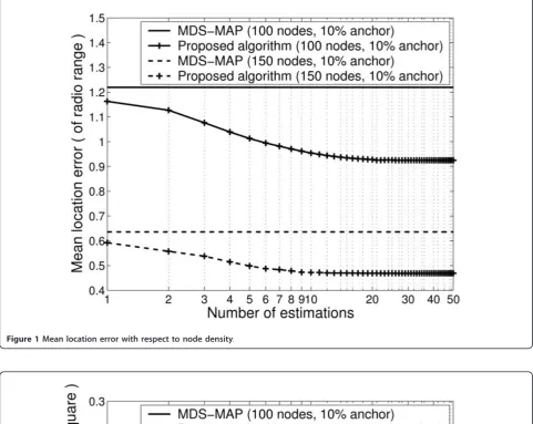
Figures 1 and 2 show the results with respect to node density. We vary the number of nodes from 100 to 150 and anchor ratio is set to 10%. All the nodes are ran-domly deployed. As can be seen in the figures, the DV-Hop and MDS-MAP have lower MLEs as more nodes
are deployed. Both algorithms assume that hop count between nodes is proportional to the distance. However, in sparse networks, holes are easily observed and lead to an increase of hop count between nodes; as a result, nodes overestimate the distances to others. While, the size and number of holes are reduced as the network becomes denser. This is why both algorithms perform better in dense networks. Each MLE of the two algo-rithms is close to another. With the proposed algorithm using the DV-Hop for the initial estimation, the MLEs decrease as the number of estimations increases. The
MLEs converges to 0.92 dmaxand 0.45dmaxin networks
with 100 and 150 nodes, respectively, after approxi-mately 10 estimations. The MLEs of the proposed algo-rithm decrease 0.27dmaxand 0.12dmaxfrom the initial
in 100 and 150 nodes, respectively. The GVLs also con-verge after 10 estimations and reductions in the GVL of the proposed algorithm are approximately 0.16d2max and
0.06d2max in 100 and 150 nodes, respectively. Due to the
assumption that hop count is proportional to the dis-tance, differences in the GVL of the DV-Hop and MDS-MAP are small and larger GVL is obtained with sparser network.
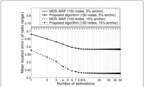
5.2.2 Anchor ratio
In this simulation, we capture the effect of anchors on the performance. The results are shown in Figures 3 and 4. In the experimental region, 150 nodes are ran-domly deployed and we vary anchor ratio from 5 to 15%. The results of the MDS-MAP are nearly identical irrespective of anchor ratio, whereas the DV-Hop has lower MLE when anchor ratio is higher. This is because there is a fundamental difference in location estimation of the two algorithms. The DV-Hop is based on the tri-or multi-lateration in which the location of each node is determined only with the distance estimations to anchors. The MDS-MAP uses the multidimensional scaling that produces a solution with the distance esti-mations to all other nodes. When anchor ratio is 5%, the proposed algorithm has 0.08 dmax and 0.065d2max
reductions on the MLE and GVL, respectively. The reductions on the MLE and GVL of the proposed algo-rithm are 0.15dmaxand 0.05d2max respectively with 15%
anchor ratio. The rate of reduction on the MLE grows as anchor ratio increases. The reason is that more nodes have perfectly accurate knowledge for their location esti-mations; as more anchors assist more nodes in locating themselves. However, the GVLs converge to a point of
0.065d2
max irrespective of the anchor ratio. Compared
Figure 1Mean location error with respect to node density.
Figure 3Mean location error with respect to anchor ratio.
the GVL is similar, that is, it is determined by node density.
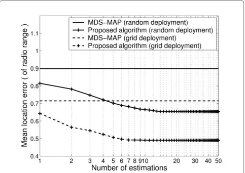
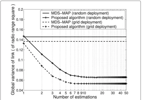
5.2.3 Node deployment
We classify node deployment methods as random deployment for anisotropic topology and grid deploy-ment for isotropic topology. According to the random deployment, nodes are randomly deployed with a uni-form distribution. Thus, nodes have heterogeneous links. Most of the nodes may be placed in a specific region; some parts of the experimental region are cov-ered with only a few nodes or none. On the other hand, nodes are deployed on grids in the grid deployment. The node degree (i.e., number of neighbors) of each node is close to the mean node degree of the network. The distances between neighbors are also similar. In this simulation, we deploy 120 nodes with 10% anchor ratio according to the node deployment methods.
The results are shown in Figures 5 and 6. With the assumption mentioned above, the DV-Hop and MDS-MAP work well on the grid deployment rather than on the random deployment. When node distribution fol-lows the random deployment, the MLE and GVL of the
proposed algorithm decrease 0.15 dmaxand 0.08d2max
from the initial, respectively. The reductions on the
MLE and GVL of the proposed algorithm are 0.17dmax
and 0.08d2
max with the grid deployment, respectively.
The decrements on the MLE and GVL of the proposed algorithm according to the two methods are similar. However, when nodes are deployed with the grid deployment, the MLE and GVL of the proposed algo-rithm on the grid deployment reach convergence points after 6 estimations. In this section, we showed that the MLE can be diminished by reducing the variance of links between one-hop neighbors through extensive simulations. The proposed algorithm reaches stable states approximately after 10 estimations. Here, the number of estimations indicates communication cost. Thus, the proposed algorithm spends communication cost ofO(S) for a refinement after start-up.
The DV-hop has a low computational complexity compared to proposed algorithm. It is because a solu-tion is calculated at one calculasolu-tion without iterasolu-tion in the DV-hop. In case of the MDS-MAP and our
algorithm, both the algorithms find out a solution itera-tively. Thus, the computational complexity of the algo-rithms is higher than the DV-hop. The MDS-MAP produces a map that minimizes the difference among links of all pairs of nodes in the network. In the process, location estimates are refined iteratively. Since dissimila-rities between all pairs of nodes are required to make the map, communication cost and computational com-plexity increase with respect to the number of nodes. Our algorithm also refines location estimates iteratively by mass spring method and Kalman filtering to mini-mize variance of links of all pairs of one-hop neighbors. The computational complexity is also increased with respect to the number of nodes. Thus, the proposed algorithm and MDS-MAP have the similar computa-tional complexity and convergence rate.
6 Conclusion
In wireless ad hoc networks, many range-free schemes have been proposed to solve the localization problem by using connectivity between nodes as a distance metric. However, the connectivity cannot sufficiently reflect the
distance between nodes. As a result, errors are produced in location estimations. We proposed a novel range-free algorithm using the mass spring method and Kalman fil-tering to find the location of a node which minimizes variance of links to all its neighbors. To the best of authors’knowledge, this is the first approach combining the mass spring method and Kalman filtering for range-free localization. Through simulations, we showed that location error is reduced as the variance of links decreases. We also showed that the proposed algorithm adapts well to various scenarios. However, the proposed algorithm has a drawback of heavy communication cost for information exchange. Reducing communication cost remains as our future study.
Acknowledgements
A preliminary version of this article was appeared in KICS (Korea Information and Communications Society) Journal 2010. This version includes a fully remodeled refinement algorithm and an extended analysis of the simulation results including other approach.
Competing interests
Received: 9 July 2011 Accepted: 30 April 2012 Published: 30 April 2012
References
1. B Rao, L Minakakis, Evolution of mobile location-based services. Commun ACM.46(12), 61–65 (2003). doi:10.1145/953460.953490
2. CY Chong, SP Kumar, Sensor networks: evolution, opportunities, and challenges. Proc IEEE.91(8), 1247–1256 (2003). doi:10.1109/ JPROC.2003.814918
3. S Lee, C Lee, Broadcasting in Mobile Ad-Hoc Networks, inMobile Ad-Hoc Networks: Protocol Design, ed. by Wang X (InTech, India, 2011), pp. 579–594 4. A Nemra, N Aouf, Robust INS/GPS sensor fusion for UAV localization using
SDRE nonlinear filtering. IEEE Sensors J.10(4), 789–798 (2010)
5. D Dardari, A Conti, U Ferner, A Giorgetti, MZ Win, Ranging with ultrawide bandwidth signals in multipath environments. Proc IEEE.97(2), 404–426 (2009)
6. SD Chitte, S Dasgupta, Z Ding, Distance estimation from received signal strength under log-normal shadowing: bias and variance. IEEE Signal Process Lett.16(3), 216–218 (2009)
7. X Li, K Pahlavan, Super-resolution TOA estimation with diversity for indoor geolocation. IEEE Trans Wirel Commun.3, 224–234 (2004). doi:10.1109/ TWC.2003.819035
8. L Yang, KC Ho, Alleviating sensor position error in source localization using calibration emitters at inaccurate locations. IEEE Trans Signal Process.58(1), 67–83 (2010)
9. Y Shen, MZ Win, On the accuracy of localization systems using wideband antenna arrays. IEEE Trans Commun.58(1), 270–280 (2010)
10. Y Shen, MZ Win, Fundamental limits of wideband localization-Part I: a general frame-work. IEEE Trans Inf Theory.56(10), 4956–4980 (2010) 11. D Niculescu, B Nath, Ad Hoc Positioning System (APS). inProc of IEEE
GLOBECOM, Texas, USA.5, 2926–2931 (2001)
12. Y Wang, X Wang, Range-free localization using expected hopprogress in wireless sensor networks. IEEE Trans Parallel Distrib Syst.20(10), 1540–1552 (2009)
13. A Howard, MJ Mataric, G Sukhatme, Relaxation on a mesh: a formalism for generalized localization. inProc of IROS, Hawaii, USA.2, 1055–1060 (2001) 14. J Sheu, P Chen, C Hsu, A distributed localization schemefor wireless sensor
networks with improved grid-scan and vector-based refinement. IEEE Trans Mobile Comput.7(9), 1110–1123 (2008)
15. NB Priyantha, H Balakrishnan, E Demaine, S Teller, Anchor-free distributed localization in sensor networks. Tech Rep 892, MIT Lab For Comput Sci (2003)
16. AS Paul, EA Wan, RSSI-based indoor localization and tracking using sigma-point kalman smoothers. IEEE J Sel Top Signal Process.3(5), 860–873 (2009) 17. MS Grewal, AP Andrews, Kalman Filtering: Theory and Practice Using
Matlab, (John and Wiley sons, Ltd., New Jersey, USA, 2001) 18. R Negenborn, Robot Localization. Kalman Filters, M.S. thesis, Utrecht
University http://www.negenborn.net (2003)
19. J Eckert, F Villanueva, R German, F Dressler, Distributed mass-spring-relaxation for anchor-free self-localization in sensor and actor networks. in Proc of IEEE ICCCN, Hawaii, USA 1–8 (2011)
20. Y Shang, W Ruml, Y Zhang, M Fromherz, Location from MereConnectivity. inProc of ACM MobiHoc, Maryland, USA 201–212 (2003)
21. Y Shang, W Ruml, Improved MDS-based localization. inProc of IEEE INFOCOM, Hongkong.4, 2640–2651 (2004)
22. N Bulusu, J Heidemann, D Estrin, GPS-less low-cost outdoor localization for very small devices. IEEE Personal Commun.7(5), 28–34 (2000). doi:10.1109/ 98.878533
23. AA Kannan, B Fidan, G Mao, Robust distributed sensor network localization based on analysis of flip ambiguities. inProc of IEEE GLOBECOM, LA, USA 1–6 (2008)
doi:10.1186/1687-1499-2012-152
Cite this article as:Leeet al.:Wireless sensor network localization with connectivity-based refinement using mass spring and Kalman filtering. EURASIP Journal on Wireless Communications and Networking2012
2012:152.
Submit your manuscript to a
journal and benefi t from:
7Convenient online submission
7Rigorous peer review
7Immediate publication on acceptance
7Open access: articles freely available online
7High visibility within the fi eld
7Retaining the copyright to your article