Introducing localized constraints in global geomagnetic field modelling
Vincent Lesur
British Geological Survey, Murchison House, West Mains Road, Edinburgh, EH9 3LA, UK
(Received November 18, 2004; Revised August 16, 2005; Accepted August 25, 2005; Online published April 14, 2006)
A set of functions is defined that can be used for modelling the internal part of the geomagnetic field. These functions are represented in term of spherical harmonics of a given maximum degreeLand are centred at specific latitudes and longitudes. The number of functions needed and the positions of their centres are such that any potential field of maximum spherical harmonic degreeL can be modelled. Formulae are obtained to transform between the potential field representation using these functions and a classic spherical harmonic representation. The shape of these functions can be optimized to make them reasonably localized, and from there it is shown how a localized constraint can be applied to an internal geomagnetic field model. The technique is demonstrated by means of models built from a few months of the Swarm mission synthetic data set.
Key words:Geomagnetism, Geomagnetic Field, Swarm, Localized constraints, wavelets.
1.
Introduction
One of the major difficulties when building a geomag-netic field model is to estimate the weights to be given to the different data sets and, in the data sets themselves, the appropriate weight for each data value. The data with un-correlated errors should be weighted by the inverse of their variances but usually these variances are not known. Fur-thermore, geomagnetic field models do not generally model all the sources of magnetic field and the data weights should take into account the part of the signal that is not modelled. Again, estimating accurately the amplitude of these signals is very difficult, if not impossible.
The usual approach when building spherical harmonic models of the geomagnetic field from satellite data is to weight the data to take into account the higher data density close to the poles and the increase in noise level at high latitude. This approach, however, is not always satisfactory. The problem would not be so acute if, in place of a spherical harmonic representation, local basis functions were used. In this case, localized noisy data would not have any influence on a local basis function parameter situated far away and, if necessary, a constraint could be applied locally to control the field model behaviour wherever there are noisy, sparse or poor quality data.
Local basis functions can be seen as a special case of wavelets and theoretical work has been done to develop wavelets on a sphere (Freedenet al., 1998). There are very few models of the internal geomagnetic field built using wavelets. Maier and Mayer (2003) present an application to the crustal magnetic field. Another example is presented in Holschneideret al.(2003) where the authors used Poisson multipole wavelets that contain all spherical harmonic de-grees. In the present work we develop a set of functions for the representation of the internal magnetic field where each function can be described with only spherical harmonics of
c
NERC, 2006. All Rights Reserved.
degrees less than or equal to a given valueL. These func-tions are a special case of “band-limited wavelets” (Free-denet al., 1998). We choose to limit the maximum spher-ical harmonic degree of the functions to have good control on the downward continuation process associated with the use of satellite data. Because our functions do not contain spherical harmonic degrees larger than L, we define and place them on the sphere in such a way that any harmonic function of spherical harmonic degree less than or equal to Lcan be represented. Therefore, we will see that it is easy to transform between a spherical harmonic representation of a potential field and a representation using our set of func-tions. Indeed, since we have only a finite number of spheri-cal harmonic degrees we can only build “quasi-lospheri-cal” func-tions that have very small amplitude outside a given latitude and longitude window (but not zero as would be expected for truly local functions). However, we will see that we can make them reasonably localized, and as a result, it is easy to implement localized constraints.
In the next section, the theory is presented, and in the third section an example is given of an application using the Swarm synthetic satellite data set (Olsenet al., 2006).
2.
Theory
A general description of wavelets on the sphere and, more specifically, band-limited wavelets can be found in Freedenet al.(1998), but in the following we concentrate on the representation we choose. Then, formulae are estab-lished to transform a spherical harmonic representation into the new system of representation, and conversely. The func-tions used for the representation are then optimized to make them as local as possible. Finally localized constraints are introduced.
Let H aL()be the space of the restriction of all har-monic functions of maximum degreeLto the unit sphere. Ifg(θ, ϕ)is a function of H aL(), it can be expressed as a linear combination of Schmidt normalized spherical
monicsYlm(θ, ϕ)1:
The negative orders (m < 0) are associated with sin(mϕ) terms, whereas zero or positive orders (m ≥ 0) are associ-ated with cos(mϕ)terms. Theg˜ml are calculated by
integra-We want to use an alternative representation forg(θ, ϕ):
g(θ, ϕ)=
i,j ˜
gi jFi jL(θ, ϕ). (3)
The functions FL
i j(θ, ϕ)are centred on a point(θi, ϕj)of the unit sphereand are defined by:
Fi jL(θ, ϕ)=
whereμis the angle between the two unit vectors pointing in the directions (θi, ϕj)and(θ, ϕ)and Pl(cosμ)are the Legendre polynomials of degreel(see Backuset al., 1996, p. 141). Obviously the functionsFL
i j(θ, ϕ)are inH aL(). where xi is the ith zero of the Legendre polynomial
PL+1(x).
This is a direct consequence of the following sampling theorem on:
Theorem-1:Letg˜lmbe the spherical harmonic coefficients of a functiong(θ, ϕ)ofH aL() (i.e.g˜lm=0 forl >L)
We do not give here a proof for this theorem that is of-ten used in geophysics (e.g., Lesur and Gubbins, 1999 or
1In our formulation we will include the spherical harmonic of zero degree
and order, but it can be excluded for geomagnetic applications.
Sneeuw, 1994). An alternative sampling theorem could be used with regular sampling both in θ andϕ (Driscoll and Healy, 1994) but twice as many functions FL
i j(θ, ϕ) would then be required. To the author’s knowledge an exact sampling theorem on the sphere requiring less than
(L+1)(2L+1)sampling points has not been established yet. By using such a theorem, one would be able to re-produce the results presented below with fewer functions FL Eq. (1) and then introducing Eq. (8) gives:
g(θ, ϕ)= expressed in terms of FL
i j(θ, ϕ), as in Eq. (3), as long as
fl =0, i.e. theFi jL(θ, ϕ)span the wholeH aL()space. It would be tempting to reduce the required number of functions FL
i j(θ, ϕ)(see for example Cui and Freeden, 1997). However, by doing so, we would not be able to es-tablish the set of Eqs. (9) and Eq. (10). It is because we are using anexactsampling theorem on the sphere that we are able to prove that theFL
i j(θ, ϕ)span the wholeH aL() space.
The (L +1)(2L +1) functions Fi jL(θ, ϕ) are not lin-early independent since the dimension of H aL()is only
(L+1)2. Therefore there is not a unique decomposition of a function ofH aL()in terms ofFi jL(θ, ϕ). Equation (10) gives a possible set ofg˜i jas a function of theg˜lm. By equat-ing Eqs. (1) and (3), multiplyequat-ing both sides byYm
1e-09 1e-08 1e-07 1e-06 1e-05 0.0001 0.001 0.01 0.1 1
0 20 40 60 80 100 120 140 160 180
Colatitude
|Potential|
|gradient along theta| |gradient along radius|
Fig. 1. Normalized absolute value of the potentialF20
00(θ, ϕ,a)and its gradients in theθandrdirections.
0.01 1 100 10000 1e+06 1e+08 1e+10
0 2 4 6 8 10 12 14 16 18 20
Power (nT^2)
Degree
Model_1
Model_2 Model_1-reference
Model_2-reference
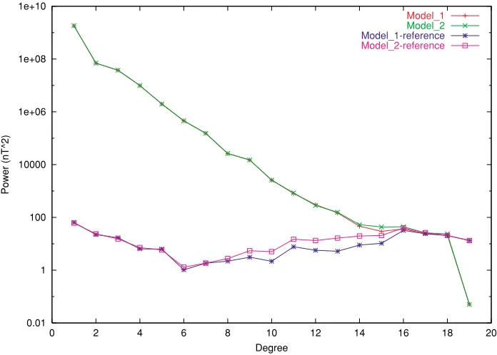
Fig. 2. Power spectra of model 1, model 2 and of their differences relative to the reference field model for 1997.5.
reciprocal formula:
˜ glm =
L+1
i=1 2L+1
j=1
˜
gi jflYlm(θi, ϕj) (11)
We now consider the problem in the whole 3-D space and define the functionFi jL(θ, ϕ,r)by:
Fi jL(θ, ϕ,r)=a L
l=0
l
m=−l
a r
l+1
flYlm(θi, ϕj)Ylm(θ, ϕ)
fl=0r ≥a (12)
Finding the best possible fl to build “local” Fi jL(θ, ϕ,r) functions is very similar to the discussion about the “δ -ness” of averaging kernels in Backus and Gilbert (1968) (see also: Backuset al., 1996, p. 153). In the present work, the fl that minimize Eq. (13) below are used, withad hoc weight function wL(θ) and associated value γ = 0.873 (in radians). This minimizes the magnitude of the gradi-ent of FL
00(θ, ϕ,a) for all θ = 0 (and not the amplitude
ofFL
00(θ, ϕ,a)because we have ultimately to model a
rel-ative to the vector pointing in the direction of their centre
(θi, ϕj). In Eq. (13), the function F00L(θ, ϕ,a)is centred on the North Pole so that it does not depend on longitudeϕ.
I =1−∂rF00L(0,0,a)
Figure 1 shows the absolute value of the poten-tial F20
00(θ, ϕ,a) and its gradients ∂θF0020(θ,0,a) and
∂rF0020(θ,0,a)as a function of colatitudeθ. These gradients decrease rapidly asμ, the angle between the two unit vec-tors pointing in the directions(θ0,0)and(θ,0), increases.
Obviously, if the maximum degreeLis increased, functions FL
00(θ, ϕ,a)can be built with gradients that decrease even
faster withμ.
In geomagnetic applications, the functions FL
i j(θ, ϕ,r) defined in Eq. (12) can be used to parameterise a magnetic field whose sources are inside a sphere of radiusa. The magnetic field is a gradient of a potential therefore:
B= −∇ lem with no unique solution (because theFL
i j(θ, ϕ)are not linearly independent) and regularization is needed. Further problems can arise if one of the fl is too small, leading to a normal equation matrix that displays (non-zero but) very small eigenvalues. Typically this will happen for large val-ues of “l” when the data acquisition surface is away from the reference surface of radiusa. For this case, again, some regularization will be needed.
ConsiderN(N ≤(L+1)(2L+1))pairs of indices{i,j} and the associated subset SN of functions Fi jL(θ, ϕ,r). A magnetic fieldB˜ is then defined by:
˜
where the g˜i j are the parameters that define the magnetic fieldBin Eq. (14). If a constraint is applied for all latitudes and longitudes onB˜, it will only have a local effect onB
as long as theNfunctionsFL
i j(θ, ϕ,r)all have their centres
(θi, ϕj)in a restricted latitude and longitude window. In the next section, an internal magnetic field model will be estimated from a data set and a measure of the roughness of its vertical component on the sphere of radius a will be minimized at high latitude. Using the definition of the functionsFL
The measure of the roughness (i.e. the measure of the am-plitude of the second tangential derivative) of the magnetic fieldB˜ vertical component on the sphere of radiusais then:
Ia =
(θt, ϕs). We have used the Schmidt normalization relation:
The model of the main magnetic field that minimizes the integral (17) is built by introducing in the least-squares scheme a damping matrix D whose elements associated with the parametersg˜i jandg˜tsare given by:
In our approach, a geomagnetic field model is defined by Eq. (14) and the damping matrix defined in (20) is used. Alternatively, the field can be modelled by a spherical har-monic representation and the damping matrix is then the same as above but right multiplied by the matrix defined in Eq. (10) and left multiplied by its transpose. In this lat-ter approach, which we would use for example to build a model of the crustal magnetic field to a high spherical har-monic degree, the advantage is a smaller number of parame-ters. Building the damping matrix would then require more work but it is straightforward.
3.
Application to a Synthetic Data Set
In this section we use the Swarm synthetic data set (Olsen et al., 2006) spanning several months in 1997 and compare models with and without local constraints. These models are also compared with the Swarm reference model for 1997.5.
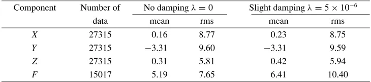
Table 1. Mean andr msmisfit to the data set for the two models.
Component Number of No dampingλ=0 Slight dampingλ=5×10⁻⁶
data mean rms mean rms
X 27315 0.16 8.77 0.23 8.75
Y 27315 −3.31 9.60 −3.31 9.59
Z 27315 0.31 5.81 0.42 5.94
F 15017 5.19 7.65 6.41 10.40
These data were fitted with a very simple geomagnetic field model:
The model is not time dependent and corresponds roughly to a snapshot model for 1997.5. The functionsFL
i j(θ, ϕ,r) are defined in Eq. (12) and the maximum spherical har-monic degree used for the internal part of the model is L =19.
This model is defined by 788 parameters (780 inter-nal and 8 exterinter-nal parameters) whereas in the equivalent “spherical harmonic only” representation only 408 parame-ters (including thel =0,m =0 internal parameter) would have been required.
The standard deviations associated with the data are de-fined by:
σ =σ0+dz(1+cos(za)) (22) where za is the zenith angle of the sun at 250 km alti-tude, the factor dz = 10 nT andσ0 = 2 nT are used for
all data. During the inversion the data are multiplied by weights proportional to the inverse of these standard devi-ations. To deal with the data density at high latitude, these weights are further divided by the number of data in roughly equal-area cells whose size at the equator was 5◦ in lati-tude and longilati-tude. Since they are selected for the northern hemisphere summer, the data at high (positive) latitudes are sparse, noisy and strongly down-weighted in the inversion process.
The model parameters are estimated using the usual least-squares iterative process:
where the superscriptidenotes theith iterate,pis the model vector (i.e. the model parameters),G(p)is the forward non-linear function used to calculate the predicted data valuesd
from a modelp,Wis a diagonal matrix whose elements are the weights described above, squared. D is the damping matrix whose non-zero elements are defined in Eq. (20) using the N =156 functions whose centres are at latitude higher than 40◦ North. λ is the usual damping parameter.
dobs is the data vector and finally, Gis the n× p matrix associated with the equations of condition (n: number of data values;p: number of model parameters):
G=
The linear system is solved using eigenvalue/eigenvector decomposition. The problem is regularised by removing the null or very small eigenvalues and their associated eigen-vectors.
It is important to understand that when only the null eigenvalues and associated eigenvectors are removed, the output solution is exactly the one that would be obtained using a spherical harmonic representation of the magnetic field if the equivalent damping is used. This is because both the(L +1)2 spherical harmonic functions of degree
smaller or equal to L and the(L +1)(2L +1)functions FL
i j(θ, ϕ,a)span exactly the same space. However, in the solutions presented below, all eigenvalues smaller than 10−8
times the largest eigenvalue were removed for the inversion of the normal equation matrix.
Two sets of model parameters were estimated in four iterations following the process (23) and their Gauss co-efficients were calculated using Eq. (11). The first set (model 1) was obtained without damping (i.e.λ =0) and the second set (model 2) was estimated with slight damp-ing: λ = 5×10⁻⁶. Table 1 gives the number of data,
mean and the rms misfit for both models. The increase in the rms misfit with the damping mainly affects, as expected, the high latitude scalar data.
Figure 2 shows the power spectrum of the two models as well as the power spectrum of their differences with respect to the underlying model used to generate the synthetic data set. The sharp drop of the model’s power at degree 19 is the result of the regularization process described above. It is interesting to note that the damping increases the power in degrees 14 and above. This is in contrast to a damping ap-plied at all latitudes and longitudes and is due to an increase in the amplitude of the zonal Gauss coefficients. Indeed a combination of zonal harmonics can generate an extremely smooth magnetic field at high latitudes.
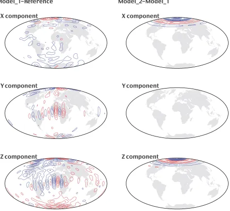
Fig. 3. Contours of the differences between, to the left, model 1 and the reference field (contour interval 10 nT, blue contours are for negative values and red positives), and to the right, model 2 and model 1 (contour interval 5 nT, blue contours are for negative values and red for positives).
between model 2 and model 1 where the contour interval is now 5 nT. These differences are large exclusively over the area where the damping was applied. Residual small differences, less than 5 nT, are present over the rest of the spherical surface in all components. It can be seen that the damping affects mainly the zonal Gauss coefficients, which was to be expected with the simple geometry and location of the damping area.
4.
Conclusion
We have presented a technique for modelling the inter-nal part of the geomagnetic field based on “quasi-local” functions. These functions are band-limited (i.e. they are built from a set of spherical harmonics with a given maxi-mum degreeL) which provides better control of the down-ward continuation of satellite data. The locations of these functions are set such that any harmonic functions of maxi-mum degreeL can be represented with these “quasi-local” functions. The consequence is that any spherical harmonic
model of the internal magnetic field can be easily trans-formed into a representation using the quasi-local functions, and conversely. The simplicity of these two transformations is the main advantage of this technique over an approach us-ing “non-band-limited” wavelets or a truly local representa-tion such as spherical cap harmonics.
These functions share the flexibility of other types of wavelets and should be well suited for building global or regional models of the crustal magnetic field in the presence of regional noise or un-modelled signal. However, in this work these functions were used specifically to introduce a localized constraint in a global magnetic field modelling process and we have shown how this local constraint can be applied to global spherical harmonic modelling. The technique was successfully tested on a data set built for the Swarm end-to-end simulator study.
the permission of the Executive Director of the British Geological Survey (NERC).
References
Backus, G. and J. F. Gilbert, The resolving power of gross Earth data,
Geophysical Journal of the Royal Astronomical Society,16, 169–205, 1968.
Backus, G., R. Parker, and C. Constable,Foundations of Geomagnetism, Cambridge University Press, New York, 1996.
Cui, J. and W. Freeden, Equidistribution on the sphere,SIAM J. Sci. Com-put.,18(2), 595–609, 1997.
Driscoll, J. R. and D. M. Healy, Computing Fourier transforms and convo-lutions on the 2-sphere,Adv. Appl. Maths,15, 202–250, 1994. Freeden, W., T. Gervens, and M. Schreiner,Constructive Approximation
on the Sphere, with Applications to Geomathematics, Clarendon Press, Oxford, 1998.
Holschneider, M., A. Chambodut, and M. Mandea, From global to re-gional analysis of the magnetic field on the sphere using wavelet frames,
Physics of the Earth and Planetary Interiors,135, 107–124, 2003. Lesur, V. and D. Gubbins, Evaluation of fast spherical transforms for
geophysical applications,Geophysical Journal International,139, 547– 555, 1999.
Maier, T. and C. Mayer,Multiscale downward continuation of CHAMP FGM-data for crustal field modelling. First CHAMP Mission Results for Graviy, Magnetic and Atmospheric Studies, edited by Reigber, L¨uhr, and Schwintzer, Springer Verlag, ISBN 3-450-00206-5, pp. 288–295, 2003.
Olsen, N., R. Haagmans, T. J. Sabaka, A. Kuvshinov, S. Maus, M. E. Pu-rucker, M. Rother, V. Lesur, and M. Mandea, TheSwarmEnd-to-End mission simulator study: A demonstration of separating the various con-tributions to Earth’s magnetic field using synthetic data,Earth Planets and Space,58, this issue, 359–370, 2006.
Sabaka, T. J., N. Olsen, and M. I. Purucker, Extending comprehensive models of the Earth’s magnetic field with Ørtsed and CHAMP data,
Geophys. J. Int.,159, 521–547, 2004.
Sneeuw, N., Global spherical harmonic analysis by least squares and nu-merical quadrature methods in historical perspective,Geophysical Jour-nal InternatioJour-nal,118, 707–716, 1994.