Dynamic behaviors of a discrete time predator–prey bioeconomic system

(1)

R E S E A R C H

Open Access

Dynamic behaviors of a discrete-time

predator–prey bioeconomic system

Weiyi Liu

*

_{, Donghan Cai and Jie Shi}

*_{Correspondence:} [email protected] School of Mathematics and Statistics, Wuhan University, Wuhan, P.R. China

Abstract

Bifurcation and chaotic behavior of a discrete-time singular bioeconomic system are investigated. First, the traditional catch equation is modified after accounting for the handling time of the catch in a singular bioeconomic system. To discover the richer dynamics compared with the continuous form, the proposed system is considered difference scheme. Specially, the tangent space local parameterization condensed method for DAEs is generalized. The new local parameterization method is sufficiently general to be applicable to this type of discrete singular system. Also the dynamic behaviors of the system are investigated, by using normal form theory, center manifold theorem and bifurcation theory, it is shown that the system undergoes a Neimark–Sacker bifurcation and a flip bifurcation, on varying step-size in some range. In addition, numerical simulations are presented not only to illustrate our results with the theoretical analysis, but also to exhibit the complex dynamical behaviors.

MSC: Primary 37G10; secondary 39A28; 39A30

Keywords: Generalized local parameterization method; Discrete singular system; Bioeconomic system; Nonlinear harvesting rate; Stability; Codimension-one bifurcation; Chaotic behavior

1 Introduction

The study of bioeconomics has a very long history. Bioeconomics is closely related to the early development of theories in ﬁshery economics. The basic model due to Gordon (1954) and Schaefer (1957) is

dx

dt =G(x) –h(x,E),

and the instantaneous proﬁt rate is

v=ph(x,E) –cE, (1.1)

where the “catch equation”

h(x,E) =qEx (1.2)

is called the Schaefer catch–effort relation [1].xis the biomass at timet.Eis the harvesting effort, in the fishery setting, which is typically specified as the number of (standard) vessels

(2)

actively fishing at time t. The units of harvesting effort would then be Standard Vessel Units (SVU).cis the cost of effort, andpis the ex-vessel price of fish. The parameterq is a constant, called catchability, units ofqare SVU–1×(time unit)–1. Thus,qrepresents the proportion of the current stockxcaught by one standard vessel in one time unit (to normalize units, one could letq= 1). To be specific we will now use time units of days (rather than years). ThusG(x) now represents the population growth per day andhis the daily harvesting rate, both being measured in tonnes per day.

Predator–prey models with harvesting is always a hot research topic (see [2–9]). The most general form of the two-dimensional predator–prey model is Kolmogorov’s model [10]:

⎧ ⎨ ⎩

˙

x=xf(x,y),

˙

y=yg(x,y), (1.3)

herexandydenote the prey and predator populations at timet, respectively. In recent years, to analyze this model from an economic point of view, many researchers have stud-ied a class of bioeconomic systems which combine system (1.3) with prey (or predator) harvesting and (1.1), and obtained some excellent results, such as the stability of equilib-ria, limit cycle, Hopf bifurcation, saddle-node bifurcation, singular induced bifurcation (see [4–6, 8, 9, 11, 12]). It is given by

⎧ ⎪ ⎪ ⎨ ⎪ ⎪ ⎩

˙

x=xf(x,y) –h(x,E),

˙

y=yg(x,y),

v=ph(x,E) –cE,

(1.4)

hereEis the effort applied to harvesting the prey at timet. The extended model is a sys-tem of differential-algebraic equations (DAEs) with differential variablesx,yand algebraic variableE. In these literatures,h(x,E) is traditionally taken asqEx. However, the Schaefer catch–effort relation has some flaws as Ref. [13] points out:

(i) All processes affecting stock productivity (e.g., growth, mortality and recruitment) are subsumed in the effective relationship between effort and catch. This

hypothesis has been proved to be not reasonable.

(ii) The catchability coeﬃcientqis not always constant. Improvements in technology and ﬁshing power makeqoften vary through time.

(iii) The harvesting function did not account for the handling time of the catch and the competition between standard vessels which are utilized for harvesting of resource. On the contrary, evidence for a nonlinear harvest function is quite strong for a number of stocks [14].

(3)

discrete-time models can also govern eﬃcient computing models for continuous ones in order to achieve the numerical emulation. However, as far as we know, there are few stud-ies of the diﬀerence scheme of system (1.4) which represents a class of discrete singular systems and no one has considered the general method to be applied to deal with it by now.

The main objective of this paper is to investigate the dynamic behaviors of a discrete-time economic predator–prey model. The model, featuring a more realistic nonlinear har-vesting function, will give rise to some interesting dynamic behaviors, as we see in Sect. 4. The paper is organized as follows. We develop a local parameterization method based on the tangent space local parameterization of DAEs in [16] and use it to deal with the afore-mentioned discrete singular system in the next section. In Sect. 3, we analyze the stability of the fixed point. In addition, we also classify the fixed point based on the geometric properties of trajectories distribution near it. Surprisingly, little study has been done on this aspect for discrete systems. Section 4 is devoted to the main results of this paper, the proposed system is investigated as it undergoes a Neimark–Sacker bifurcation and a flip bifurcation. Section 5 contains a numerical verification of some key results. Conclusion and discussion are presented in Sect. 6.

2 Statement of model and local parameterization

Consider the scaled equation, describing a singular bioeconomic system (see [6, 9, 17–19]) with nonlinear harvesting function, as

⎧ ⎪ ⎪ ⎨ ⎪ ⎪ ⎩

˙

x=x(a–kx–y) –₁₊xE_mx,

˙

y=y(–s+x),

v=₁₊pxE_mx–cE.

(2.1)

For the practical signiﬁcance, the system (2.1) is deﬁned on the set

R3₊=(x,y,E)∈R3₊|x≥0,y≥0,E≥0,

and is subject to positive initial conditions,

x(0) > 0, y(0) > 0, E(0) > 0.

Equation (2.1) is a semi-explicit autonomous differential-algebraic equations with differ-ential index 1, ₁₊xE_mxis the harvesting function with constantmbeing related to the han-dling or processing time [17, 19]. Though this nonlinear harvesting function is more real-istic, not many researchers have used it in their studies. Form= 0 it reduces to the Schaefer catch–effort equation (1.2).

We put (x,y,E)T_X_{and use}_X

0= (x0,y0,E0)Tto denote the equilibria of (2.1). It can be

checked that system (2.1) has a unique equilibria,

X0=

s,a–ks– v

(p–cm)s–c,

(1 +ms)v (p–cm)s–c

(4)

We haveX0∈R3+, in this work, we take parameters (a,k,s,p,m,c,v) from the set

For (2.1), if derivatives are replaced by finite difference approximations, then we get the forward Euler difference scheme with step-sizeδ:

⎧

We can easily verify that the ﬁxed point of (2.3) is alsoX0. Now we will determine the local

equivalent parameterization system of (2.3).

We ﬁrst rewrite (2.1) into the constrained form [16], that is, the diﬀerential equations on the manifold,

The algebraic equation sets an invariant manifold (denoted byM) inR3_{[16] whose}

num-ber of independent coordinates is 2.E˙ is described through a derivation of the algebraic equation along the solution path with respect to timet and it is not necessary for the concrete formula as we will see later. Accordingly, (2.2) becomes the following diﬀerence algebraic equations of the constrained form:

⎧

It will be convenient to introduce some notation:

f1(x,y,E) =x+δx

a–kx–y– E

1 +mx ,

(5)

f3(x,y,E) =E+δf˜3(x,y,E),

g(x,y,E) = pxE

1 +mx–cE–v,

and the vector-valued function

f = (f1,f2)T, f˜= (f1,f2,f3)T.

In terms of the above notations, (2.5) becomes ⎧

⎨ ⎩

Xn+1=f˜(Xn),

g(Xn) = 0,

(2.6)

or in map form ⎧ ⎨ ⎩

X→ ˜f(X),

g(X) = 0.

(2.7)

Note that the form of (2.6) or (2.7) is generic (representing diﬀerence algebraic equations in constrained form). We next generalize the tangent space local parameterization method for general diﬀerential-algebraic equations in constrained form to parameterize (2.6) or (2.7). First we give a decomposition forMinR3as follows:

X–X0=U0Y+V0Y, ∀X∈M,

or

X=X0+U0Y+V0Y, ∀X∈M. (2.8)

[U0,V0] is an arbitrary order-three orthogonal matrix whose columns consist of a basis for

R3_with_U

0is 3×2 andV0is 3×1.Y:= (y1,y2)T∈R2is the coordinate associated with the

projection ofX–X0onto the column space ofU0, andY∈Ris the coordinate associated

with the projection ofX–X0onto the column space ofV0; note thatY might be locally

represented byY. Indeed,

g(X0+U0Y+V0Y) = 0.

LetG(Y,Y) =g(x0+U0Y+V0Y), therefore

detDYG(Y,Y)

=DYg(X0+U0Y+V0Y) =Dg·V0= 0,

whereDis a derivation operator. Hence, there exists a smooth map:h:R2_→_R_guaranteed

by the implicit function theorem such thatY=h(Y) locally holds. Putting it in (2.8) gives a local parameterization of the solution manifold with parameterYas follows:

(6)

where

ψ(Y) = ⎛ ⎜ ⎝

ψ1(y1,y2) ψ2(y1,y2) ψ3(y1,y2)

⎞ ⎟ ⎠.

Obviously,ψis related toh.

From (2.9) together with the ﬁrst equation of system (2.6) we get

ψ(Yn+1) =f˜

ψ(Yn),

which gives

X0+U0Yn+1+V0h(Yn+1) =f˜

ψ(Yn),

multiplying byU₀Tgives

U₀TX0+Yn+1=U0Tf˜

ψ(Yn),

that is,

Yn+1=U0Tf˜

ψ(Yn)–U₀TX0, (2.10)

or in map form

Y→U₀Tf˜ψ(Y)–U₀TX0,

which is the local parameterization of (2.7) nearX0with parameterY.

Speciﬁcally, if take

U0=

⎛ ⎜ ⎝

1 0

0 1

0 0

⎞ ⎟

⎠, V0=

⎛ ⎜ ⎝ 0 0 1

⎞ ⎟ ⎠,

then

U₀Tf˜ψ(Yn)=fψ(Yn). (2.11)

Here we see thatf˜3(X) vanishes, which is why it is not necessary to give the concrete

for-mula off˜3inE˙ of the equation of (2.4). Hence using (2.10) and (2.11), we obtain the

fol-lowing parameterization system:

Yn+1=f

ψ(Yn)–U₀TX0,

or in map form

(7)

that is,

Y→fψ(Y)– (x0,y0)T. (2.12)

Equation (2.12) is topologically equivalent, near the origin, to the diﬀerence algebraic sys-tem (2.3) in a neighborhood ofX0.

Remark2.1 The ﬁxed pointX0of (2.3) corresponds to the ﬁxed pointO(0, 0) of (2.12).

Remark 2.2 Since the form of (2.6) or (2.7) has generality, the new parameterization

method is also generic (Xncan be of arbitrary ﬁnite dimensions). Speciﬁcally, if we take the tangent space and normal vector space of solution manifold atX0 asU0 andV0,

re-spectively, then the local parameterization (2.9) reduces to the tangent space local param-eterization condensed method for DAEs in [16].

3 Fixed points classiﬁcation and stability analysis

Our goal in this section is to examine the local stability of (2.3) based upon the standard linearization technique.

Fromg(ψ(Y)) = 0 we obtain

Dg(X)Dψ(Y) = 0. (3.1)

Diﬀerentiating (2.9) with respect toyand multiplying both sides byUT

0 gives

U₀TDψ(Y) =I2. (3.2)

Combine (3.1) and (3.2) to yield

Dψ(Y) =

Dg(X) UT

0

–1

0 I2

= ⎛ ⎜ ⎝

1 0

0 1

–₍₍_p_–_cm₎_xEp_–_c₎₍₁₊_mx₎ 0 ⎞ ⎟ ⎠

for future use. Note thatDψ(Y) has nothing to do withh, so we can give the concrete form of (2.12) by a Taylor formula.

The Jacobian matrix of the system (2.12) evaluated at the origin is given by

Dfψ(y)– (x0,y0)T_(0,0)

=Df(X)|X0Dψ(Y)|(0,0)

=

f1x f1y f1E f2x f2y f2E

X0

⎛ ⎜ ⎝

1 0

0 1

– E0p

((p–cm)s–c)(1+ms) 0

⎞ ⎟ ⎠

=

1 –δs(k–₍₍_p_–_cm₎_svm_–_c₎₍₁₊_ms₎) +₍₍_p_–_cm₎_svp_–δ_c₎s2₍₁₊_ms₎ –δs δ(a–ks–₍_p_–_cmv₎_s_–_c) 1

(8)

Hence the characteristic equation associated to the Jacobian matrix is given by

F(λ) =λ2+Bλ+C= 0, (3.3)

where ⎧ ⎪ ⎪ ⎨ ⎪ ⎪ ⎩

B=δs(k–₍₍_p_–_cm₎vm_s_–_c₎₍₁₊_ms₎) –₍₍_p_–_cm₎p_s_–δsv_c₎2₍₁₊_ms₎– 2,

C= 1 +₍₍_p_–_cm₎p_s_–δsv_c₎2₍₁₊_ms₎–δs(k–₍₍_p_–_cm₎vm_s_–_c₎₍₁₊_ms₎)

+sδ2(a–ks–₍_p_–_cmv₎_s_–_c).

Puttingλ= 1 andλ= –1 inF(λ), respectively, we get

F(1) =sδ2y0=sδ2

a–ks– v

(p–cm)s–c

and

F(–1) = 4 + 2E0pδs

((p–cm)s–c)(1 +ms)2 – 2δs

k– E0m

(1 +ms)2 +δ 2_sy

0

= 4 + 2pδsv

((p–cm)s–c)2_{(1 +}_ms₎– 2δs

k– vm

((p–cm)s–c)(1 +ms)

+sδ2

a–ks– v

(p–cm)s–c .

Letλ1andλ2denote the two roots of (3.3), referred to as the eigenvalues (or multipliers)

of the fixed pointO(0, 0). We first recall the relevant definitions of topological types for fixed points (see [20]).

Deﬁnition 3.1 O(0, 0) is called

(i) a hyperbolic ﬁxed point, if the moduli of all eigenvalues do not equal 1; and (ii) a nonhyperbolic ﬁxed point, if|λ1|= 1or|λ2|= 1.

Deﬁnition 3.2 IfO(0, 0) is a hyperbolic ﬁxed point, then it is called (i) a sink, if|λ1|< 1and|λ2|< 1;

(ii) a source, if|λ1|> 1and|λ2|> 1; and

(iii) a saddle, ifλ1,2are real, with|λ1|< 1and|λ2|> 1(or|λ1|> 1and|λ2|< 1).

Moreover, we can classify ﬁxed points based on the geometric properties of trajectory distribution near them.

Deﬁnition 3.3 O(0, 0) is called

(i) a saddle, ifλ1,2are real, with|λ1|< 1and|λ2|> 1(or|λ1|> 1and|λ2|< 1);

(ii) a node, ifλ1,2are real, with|λ1,2|< 1(or|λ1,2|> 1);

(iii) a focus (sometimes called spiral point), ifλ1,2=r(cosθ±isinθ),r= 1; and

(iv) a center, ifλ1,2=cosθ±isinθ.

(9)

Lemma 3.1 Suppose that F(1) > 0,then we have

(i) |λ1|< 1and|λ2|< 1iﬀF(–1) > 0andC< 1;

(ii) |λ1|> 1and|λ2|> 1iﬀF(–1) > 0andC> 1;

(iii) |λ1|< 1and|λ2|> 1(or|λ1|> 1and|λ2|< 1)iﬀF(–1) < 0;

(iv) λ1andλ2are complex and|λ1|=|λ2|= 1iﬀB2– 4C< 0andC= 1;and

(v) λ1= –1and|λ2| = 1iﬀF(–1) = 0andB= 0, 2.

Using Lemma 3.1, we obtain the following results.

Theorem 3.1 Assuming parameters(a,k,s,p,m,c,v)∈π,system(2.3)has a unique posi-tive ﬁxed point X0and

(i) it is a sink iﬀ

4 + 2δ1– 2δ2+δ23> 0 and 1–2+δ3< 0;

(ii) it is a source iﬀ

4 + 2δ1– 2δ2+δ23> 0 and 1–2+δ3> 0;

(iii) it is a saddle iﬀ

4 + 2δ1– 2δ2+δ23< 0; and

(iv) it is nonhyperbolic if one of the following conditions is satisﬁed: (iv1) δ3=2–1and(2–1)2– 43< 0;

(iv2) 4 + 2δ1– 2δ2+δ23= 0andδ2–δ1= 2, 4.

Theorem 3.2 With the assumption of Theorem3.1,X0is

(i) a stable node iﬀ

δ(2–1) < 2 and 1 +δ1–δ2+δ23> 0;

(ii) an unstable node iﬀ

2–1< 0;

(iii) a stable focus iﬀ

(2–1)2– 43< 0 and δ3<2–1;

(iv) an unstable focus iﬀ

(2–1)2– 43< 0 and δ3>2–1,

where

1=

psv

(10)

2=s

k– vm

((p–cm)s–c)(1 +ms) ,

3=s

a–ks– v

(p–cm)s–c .

4 Bifurcation analysis

Based on the analysis of Sect. 3, we discuss a codimension-one bifurcation (Neimark– Sacker bifurcation and ﬂip bifurcation) of system (2.3) at the ﬁxed point.

4.1 Neimark–Sacker bifurcation and invariant curve First, letC= 1, then we have

s

a–ks– v

(p–cm)s–c δ

2₊ psvδ

((p–cm)s–c)2_{(1 +}_ms₎

–s

k– vm

((p–cm)s–c)(1 +ms) δ= 0.

Solving this equation gives

δ1=

2–1 3

.

We chooseδas a bifurcation parameter to discuss the Neimark–Sacker bifurcation when

δvaries in a small neighborhood ofδ1. If we considerδ∗=δ–δ1, thenδ=δ1is equivalent

toδ∗= 0.

The linearization of (2.12) has the characteristic equation atO(0, 0)

F(λ) =λ2+Bδ∗λ+Cδ∗= 0,

where ⎧ ⎪ ⎪ ⎨ ⎪ ⎪ ⎩

B(δ∗) = (δ∗+δ1)s(k–₍₍_p_–_cm₎vm_s_–_c₎₍₁₊_ms₎) – (δ

∗_+δ1)_psv

((p–cm)s–c)2₍₁₊_ms₎– 2,

C(δ∗) = 1 +₍₍_p_–_cm(δ∗₎+δ1)_s_–_c₎2psv₍₁₊_ms₎– (δ∗+δ1)s(k–₍₍_p_–_cm₎vm_s_–_c₎₍₁₊_ms₎)

+s(δ∗+δ1)2(a–ks–₍_p_–_cmv₎_s_–_c).

Let

1=

(a,k,s,p,m,c,v,δ)|(a,k,s,p,m,c,v)∈π, 0 <δ=δ1, (2–1)2< 43

.

Then, if (k,a,m,s,p,c,v,δ)∈1, the characteristic values are complex conjugate numbers λandλwith|λ|=|λ|= 1, where

λ,λ= –B(δ ∗₎

2 ±

i 2

4Cδ∗–B2_δ∗_, |_λ| δ∗=0=

C(0) = 1,

and

α=d|λ(δ ∗₎_|

dδ∗

δ∗=0

=1 2

2–1

1 +1δ1–2δ1+3δ12

=2–1

(11)

In addition, it is required that whenδ∗= 0,λm_,_λm_{= 1 (}_m_{= 1, 2, 3, 4), which is equivalent}

is a one-parameter map with parameterδ∗.

We next determine, in order to get the normal form of (4.2), the Taylor expansion of the right-hand side of (4.2) at the origin to order three, that is,

where the terms with 0 coeﬃcients are omitted. By the chain rule, we have the following:

(12)

then through the change of basis with

we can change system (4.3) into the normal form

where the nonlinear terms are

f₁(z1,z2) = (a2a11+a12σ–a12a1)z21–a12ωz1z2+a111a22z31+O

In order for system (4.4) to undergo a Neimark–Sacker bifurcation atO(0, 0), we require that the following quantity is not zero [22]:

(13)

where

γ20=

(f₁_z₁_z₁–f₁_z₂_z₂+ 2f₂_z₁_z₂) +i(f₂_z₁_z₁–f₂_z₂_z₂– 2f₁_z₁_z₂)

8 ,

γ11=

(f₁_z₁_z₁+f₁_z₂_z₂) +i(f₂_z₁_z₁+f₂_z₂_z₂)

4 ,

γ02=

(f₁_z₁_z₁–f₁_z₂_z₂– 2f₂_z₁_z₂) +i(f₂_z₁_z₁–f₂_z₂_z₂+ 2f₁_z₁_z₂)

8 ,

γ21=

(f₁_z₁_z₁_z₁+f₁_z₁_z₂_z₂+f₂_z₁_z₁_z₂+f₂_z₂_z₂_z₂) +i(f₂_z₁_z₁_z₁+f₂_z₁_z₂_z₂–f₁_z₁_z₁_z₂–f₁_z₂_z₂_z₂)

16 .

Note that here all the derivatives are taken atO(0, 0). From the above discussion, we obtain the following result.

Theorem 4.1 Assume that(a,k,s,p,m,c,v,δ)∈1and the condition(4.1)holds.If l= 0,

then the system(2.3)undergoes a Neimark–Sacker bifurcation at the ﬁxed point(x0,y0,E0)

when the bifurcation parameterδ varies in a small neighborhood ofδ1.Moreover,if l< 0

(resp.l> 0),then an attracting(resp.repelling)invariant closed curve bifurcates from the ﬁxed point forδ>δ1(resp.δ<δ1).

4.2 Flip bifurcation and chaos

We proceed to investigate the ﬂip bifurcation. For (3.3), letF(–1) = 0 we obtain

4 + 2pδsv

((p–cm)s–c)2_{(1 +}_ms₎– 2δs

k– vm

((p–cm)s–c)(1 +ms)

+sδ2

a–ks– v

(p–cm)s–c = 0.

Solving this equation gives

δ2=

2–1–

(2–1)2– 43 3

.

Here we still chooseδ as a bifurcation parameter to discuss the ﬂip bifurcation whenδ

varies in a small neighborhood ofδ2. In the same way as above, we considerδ∗=δ–δ2, then δ=δ2is equivalent toδ∗= 0. Since we would like to study the system as we varyδ∗near 0,

we treatδ∗ as a variable (which has no dependence on time) and hence the parameter-free center manifold theorem can easily be extended for a parameter-dependent sys-tem.

We begin by putting

X=x,y,E,δ∗T, Y=y1,y2,δ∗

T .

Accordingly, the local parameterization (2.9) should be rewritten as

(14)

where

Hence we study the three-dimensional extended system

Y→

As in our study of the Neimark–Sacker bifurcation, we expand the right-hand side of (4.5) in the order-three Taylor polynomial,

(15)

where

Construct an invertible matrix

(16)

˜

Now, make the translation ⎛

(17)

Having gone through these coordinate changes, the parameter-dependent center manifold of (4.7) can be approximately represented as follows:

Wc(0, 0, 0) =z1,z2,δ∗

the second formula of (4.7) and obtain

h–z1+ϕ1

Therefore, we consider the map which is (4.7) restricted to the center manifoldWc_{(0, 0),}

F:z1→–z1+d11z12+d12z1δ∗+d112z21δ∗+d122z1δ∗2+d22δ∗2+d111z31+d222δ∗3

In order for system (4.10) to undergo a ﬂip bifurcation at the origin, we require that the two quantities

do not equal zero [22]. Let

then we have the following result.

Theorem 4.2 Assuming that(a,k,s,p,m,c,v,δ)∈2.Ifα˜2= 0,then the system(2.3)

un-dergoes a ﬂip bifurcation at the ﬁxed point(x0,y0,E0)when the bifurcation parameterδ

varies in a small neighborhood ofδ2.Moreover,ifα˜2> 0 (resp.,α˜2< 0),then the period-2

(18)

5 Numerical simulations

In this section, we give two examples to illustrate our theoretical analysis.

Example5.1 (Neimark–Sacker bifurcation) Here we present a numerical analysis of the

proposed system (2.3) with the following artiﬁcially chosen data:a= 4,k= 1,s= 2,p= 1, m= 0.1,c= 1 andv= 0.6 with (a,k,s,p,m,c,v)∈π. It is easy to verify that the system (2.3) has a unique ﬁxed point (2, 1.25, 0.9) andδ1= 0.125.

The multipliers of the positive ﬁxed point areλ±≈0.9805±0.1967iwith|λ±|= 1 and

α = 0.1563 > 0. SinceH= 0.0391= 2, 3, 4, the condition (4.1) holds. Then, using The-orem 4.1, the system (2.3) undergoes a Neimark–Sacker bifurcation at the ﬁxed point (2, 1.25, 0.9) withl= 0.0017 > 0.

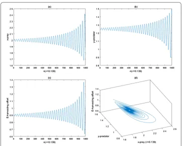
Figures 1, 2 and 3 reveal that the ﬁxed point (2, 1.25, 0.9) of (2.3) is unstable for δ= 0.125 + 0.0014 and becomes stable forδ= 0.125 – 0.035, and a repelling limit cycle appears around it atδ= 0.125 – 0.0001.

Example5.2 (Flip bifurcation) Fixa= 16,k= 4,s= 3.9,p= 7,m= 1,c= 1 andv= 1 and the ﬁxed point (3.9, 0.3554, 0.2188) with (a,k,s,p,m,c,v)∈π. After computation we get the following quantities:

δ2= 0.1294,

˜

α1= –0.1792,

˜

α2= 0.0022 – 2×6.8573×10–6> 0.

(19)

Figure 2 δ=δ1– 0.0001. An repelling invariant closed curve bifurcates from the ﬁxed point (2, 1.25, 0.9)

(20)

Figure 4(a) Bifurcation diagram in (δ,x) plane. (b) Bifurcation diagram in (δ,y) plane. (c) Bifurcation diagram in (δ,E) plane. (d) Largest Lyapunov exponents corresponding to (a), (b), and (c)

Figures 4(a), 4(b) and 4(c) reveal that the ﬁxed point is stable forδ< 0.1294, and loses its stability at the ﬂip bifurcation parameter valueδ= 0.1294. We also observe that there is a cascade of period doubling bifurcations. The largest Lyapunov exponents corresponding to Figs. 4(a), 4(b) and 4(c) are computed in Fig. 4(d).

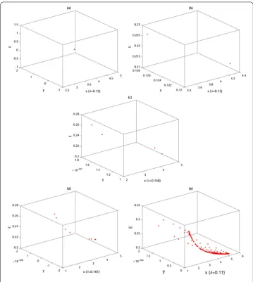
Figure 5 shows the phase portraits which are associated with Figs. 4(a), 4(b) and 4(c). For

δ∈(0.12, 0.1616), there are orbits of period 2, 4, 8, . . . . Whenδ= 0.1616, one can see that the largest Lyapunov exponent is positive, thereby conﬁrming that the system is chaotic. And then forδ∈(0.1616, 017) some largest Lyapunov exponents are negative, indicating the existence of periodic windows in the chaos region.

6 Conclusion

The present paper is concerned with the dynamics of a discrete-time economic predator– prey system in the presence of a type of nonlinear harvesting function. We find the fixed point and its stability. Most interestingly, we have seen that our results reveal a far richer dynamics of the discrete model compared with the continuous one proposed in [9], in-cluding an invariant circle, cascades of period-doubling bifurcation and chaotic sets. We confirm the complexity of the dynamic behavior by computing the largest Lyapunov ex-ponents. This paper extends our previous works (see [8, 9]) and provides a sufficiently general parameterization method for a wide range of discrete singular systems.

(21)

Figure 5Phase portraits for diﬀerent values ofδcorresponding to Fig. 4. (a)δ= 0.12, (b)δ= 0.13, (c)δ= 0.158, (d)δ= 0.161, (e)δ= 0.17

is a sufficient criterion for the existence of chaos. If the fixed point of system (2.3) is a snap-back repeller under certain parameter conditions, then one can conclude that the system is chaotic in the Marotto sense. Furthermore, various feedback controls can be implemented for controlling the bifurcation and chaos in the system (2.3), which should be useful for fishery management control and biological conversion. Space prevents that discussion here, but these issues will be the topics of our future research.

Acknowledgements

The authors wish to express their gratitude to the editors and reviewers for the helpful comments. This research is supported by National Natural Science Foundation of China under grant No. 71271158.

Competing interests

The authors declare that they have no competing interests.

Authors’ contributions

(22)

Publisher’s Note

Springer Nature remains neutral with regard to jurisdictional claims in published maps and institutional aﬃliations.

Received: 25 January 2018 Accepted: 5 April 2018

References

1. Clark, C.W.: Mathematical Bioeconomics: The Optimal Management of Renewable Resources. Wiley, New York (2010) 2. Chen, B.S., Chen, J.J.: Complex dynamic behaviors of a discrete predator–prey model with stage structure and

harvesting. Int. J. Biomath.10(1), 1–25 (2017)

3. Gupta, R.P., Chandra, P.: Dynamical properties of a prey–predator–scavenger model with quadratic harvesting. Commun. Nonlinear Sci. Numer. Simul.49, 202–214 (2017)

4. Li, M., Chen, B.S., Ye, H.W.: A bioeconomic diﬀerential algebraic predator–prey model with nonlinear prey harvesting. Appl. Math. Model.42, 17–28 (2017)

5. Liu, C., Lu, N., Zhang, Q.L.: Dynamical analysis in a hybrid bioeconomic system with multiple time delays and strong Allee eﬀect. Math. Comput. Simul.136, 104–131 (2017)

6. Liu, W., Fu, C.J., Chen, B.S.: Hopf bifurcation and center stability for a predator–prey biological economic model with prey harvesting. Commun. Nonlinear Sci. Numer. Simul.17(10), 3989–3998 (2012)

7. Liu, W., Jiang, Y.L.: Bifurcation of a delayed Gauss predator–prey model with Michaelis–Menten type harvesting. J. Theor. Biol.438, 116–132 (2018)

8. Liu, W.Y., Fu, C.J., Chen, B.S.: Stability and Hopf bifurcation of a predator–prey biological economic system with nonlinear harvesting rate. Int. J. Nonlinear Sci. Numer. Simul.16(6), 249–258 (2015)

9. Liu, W.Y., Li, B.W., Fu, C.J., Chen, B.S.: Dynamics of a predator–prey ecological system with nonlinear harvesting rate. Wuhan Univ. J. Nat. Sci.20(1), 25–33 (2015)

10. Kolmogorov, A.N.: Sulla teoria di Volterra della Lotta per l’esistenza. G. Ist. Ital. Attuari7, 74–80 (1936) (in Italian) 11. Santra, P., Mahapatra, G.S., Pal, D.: Analysis of diﬀerential-algebraic prey–predator dynamical model with super

predator harvesting on economic perspective. Int. J. Dyn. Control4, 266–274 (2016)

12. Zhang, X., Zhang, Q.L.: Bifurcation analysis and control of a class of hybrid biological economic models. Nonlinear Anal. Hybrid Syst.3, 578–587 (2009)

13. Seijo, J.C., Defeo, O., Salas, S.: Fisheries Bioeconomics: Theory, Modelling and Management. Fao Fisheries Technical Papers, vol. 368. Food and Agriculture Organization of the United Nation, New York (1998)

14. Shelton, S.J., Myers, R.A., Dunn, A.: Is catch-per-unit eﬀort proportional to abundance? Can. J. Fish. Aquat. Sci.58, 1760–1772 (2001)

15. Kot, M.: Elements of Mathematical Ecology. Cambridge University Press, Cambridge (2001)

16. Potra, F.A., Yen, J.: Implicit numerical integration for Euler–Lagrange equations via tangent space parametrization. Circuits Syst. Signal Process.19(1), 77–98 (1991)

17. Agnew, T.T.: Optimal exploitation of a ﬁshery employing a nonlinear harvesting function. Ecol. Model.6, 47–57 (1979) 18. Fred, B., Carlos, C.C.: Mathematical Models in Population Biology and Epidemiology. Springer, New York (2011) 19. Goh, B.S.: Management and Analysis of Biological Populations. Developments in Agricultural and Managed-Forest

Ecology. Elsevier, Amsterdam (1980)

20. Wiggins, S.: Introduction to Applied Nonlinear Dynamical Systems and Chaos. Springer, New York (2003)

21. Liu, X.L., Xiao, D.M.: Complex dynamic behaviors of a discrete-time predator–prey system. Chaos Solitons Fractals32, 80–94 (2007)

22. Guckenheimer, J., Holmes, P.: Nonlinear Oscillations, Dynamical Systems, and Bifurcations of Vector Fields. Springer, New York (2002)