R E S E A R C H
Open Access
Numerical solution of advection–diffusion
type equation by modified error correction
scheme
Soyoon Bak
1, Philsu Kim
1, Xiangfan Piao
1and Sunyoung Bu
2**Correspondence:
2Department of Liberal Arts, Hongik
University, Sejong, Republic of Korea Full list of author information is available at the end of the article
Abstract
In this paper, we consider a numerical solution for nonlinear advection–diffusion equation by a backward semi-Lagrangian method. The numerical method is based on the second-order backward differentiation formula for the material derivative and the fourth-order finite difference formula for the diffusion term along the characteristic curve. A modified error correction scheme is newly introduced to efficiently find the departure point of the characteristic curve. Through several numerical simulations, we demonstrate that the proposed method has second and third convergence orders in time and space, respectively, and is efficient and accurate compared to existing techniques. In addition, it is numerically shown that the proposed method has good properties in terms of energy and mass conservation.
Keywords: Semi-Lagrangian method; Advection–diffusion equations; Burgers equations
1 Introduction
The nonlinear advection–diffusion type equation is one of the popular and important models describing many phenomena derived from various areas of mathematical physics and engineering fields such as gas dynamics, hydrodynamics, shock waves, heat conduc-tion and so on. Also, the type of equaconduc-tion represents the Burgers equaconduc-tion, the heat con-duction equation, the nonlinear Schrödinger equation, the Navier–Stokes equation, etc. Hence, the development of efficient and accurate algorithms for solving the equations is of great importance in the computational fluid dynamics community and has been widely studied by many researchers. To solve theses equations, there has become a great quantity of research available [1–14] in recent decades. In particular, the error correction method (ECM) [15, 16] for solving the characteristic curve in the backward semi-Lagrangian method (BSLM) [17,18] was recently developed. This method solves a problem implic-itly along the characteristic curves of fluid particles in the opposite direction with large time steps, which is the main advantage of the BSLM [17,19]. Also, the method does not only have second and third convergence orders in time and space, respectively, but also does not have any iterative processes required to solve a nonlinear initial value problem (IVP) for departure points. To discretize the material derivative and the diffusion term along the characteristic curve in the BSLM framework, the backward difference formula
(BDF2) and the fourth-order finite difference method (FDM) [20] are applied, respectively. The departure point of the characteristic curve is found by the ECM.
The aim of this article is to introduce newly a modified ECM instead of simply using the conventional ECM, motivated by the success of the ECM combined with the BSLM. To do this, we firstly present a modified Euler polygon, for the consideration of the phys-ical domains in which the particles can move (see Sect.3for more information). In ad-dition, boundary values are calculated by the same fourth-order finite difference scheme, unlike previous work that used a lower order scheme for boundary conditions. More-over, to reduce the computational cost, the proposed scheme approximates the Jacobian value as a fixed one while maintaining the scale of the error, whereas the conventional ECM once again performs the interpolation with the derivatives of the original interpo-lation function. The interpointerpo-lation for Jacobian in the conventional ECM required consid-erable computational cost since it occurs in every spatial variables at each time step. As a simple model to show this technique effectively, we apply the proposed method to the one-dimensional and the two-dimensional Burgers equations. Through several numerical simulations, it is shown that the proposed method has second temporal and third spatial convergence orders. Further, we discuss the energy and the mass conservation properties and numerically show a good performance on these properties.
The remainder of this paper is organized as follows. In Sect.2, the BSLM based on the FDM and the BDF2 is reviewed for the Burgers equations. In Sect.3, we introduce a mod-ified error correction technique to solve the highly nonlinear IVP. Three test problems are numerically solved in Sect.4in order to demonstrate the accuracy and the efficiency of the proposed method. Finally, conclusions are given in Sect.5.
2 Backward semi-Lagrangian method
This section aims to give brief descriptions for the BSLM based on both the FDM and the BDF2 for the one-dimensional case and the system of Burgers equations.
2.1 One-dimensional Burgers equation
As a model problem, we consider the one-dimensional Burgers equation described by
ut+uux=νuxx, xL<x<xR, 0 <t≤T, (1)
with the boundary and the initial conditions given by ⎧
⎨ ⎩
u(t,xL) =g1(t), u(t,xR) =g2(t), t> 0,
u(0,x) =u0(x), x∈[xL,xR],
where ν> 0 is the coefficient of kinematic viscosity. Here,u0(x) and gk(t) (k= 1, 2) are
assumed to be sufficiently smooth functions for the existence and the uniqueness of the solution [21,22]. The solutionumay represent a temperature for heat transfer or a species concentration for mass transfer at positionxand timetwith the advection velocityu.
From the Lagrangian view, consider the characteristic curveπ(xi,tn+1;t) satisfying the
following IVP with an initial valueπ(x,s;s) =x:
dπ(x,s;t) dt =u
whereu(t,·) is the solution of (1). Then the material derivative DtDu(t,π(x,s;t)) satisfies
which is valid along the characteristic curveπ(x,s;t). Solving these two equations (2) and (3) simultaneously, the solutionuof (1) can be obtained.
For further discussion, we introduce uniform discretizations of the temporal and the spatial domains as follows:
tn=nh (0≤n≤N), xi=xL+ix (0≤i≤Mx), (4)
whereh:=T/Nandx:= (xR–xL)/Mxare the temporal step and the spatial grid sizes, respectively. Additionally, to approximate the first and the second-order partial derivatives in the considered backward semi-Lagrangian algorithm, we introduce the fourth-order finite difference weight matrices of sizeMx:=Mx+ 1 (see [20]) as follows:
x andWx2can be obtained by using a five point finite difference scheme [20] at the interior points and one-side method for points near the boundary. Using these matrices, the partial derivatives of a smooth functionf can be expressed in matrix form as follows: proposed scheme,Wx1 andWx2 are used for the interpolation scheme and the diffusion term, respectively.
we denoteun(xi) :=u(tn,xi) and its approximation byUn
i for eachxiat timet=tn. In ad-dition, we introduce the notations Un:= [Un
0,U1n, . . . ,UMnx]
T andU˜n:= [Un
1,U2n, . . . ,UMnx]T
forMx:=Mx– 1 and the superscriptT denotes the transpose. Here, we assume that the approximationsUk
i (k≤n) have been previously calculated at all grid points. After evalu-ating (3) at point (t,x) = (tn+1,xi) and applying the BDF2 for the material derivative in the left hand side of (3), we get the following formula:
un+1(xi) –μ˜unxx+1(xi) =
By applying the finite difference formula (5) withm= 2 to the diffusion term of (6), we get the semi-discretization system in matrix form as follows:
AU˜n+1= dn+1+μbn+1,
whereIdenotes an identity matrix of sizeMxandW˜x2is the matrix constructed fromWx2 by taking the interior elements (i,j) = (1 :Mx, 1 :Mx).
For the full-discretization of (7), letπin+1,kbe an approximation of the departure position π(xi,tn+1;tk) of grid point (tn+1,xi) at each time steptk, which are discussed in detail in Sect.3. Because these departure points generally do not coincide with any grid points and we only know the approximate values on the grid points att≤tn, a proper interpolation method is needed. In the proposed scheme, the Hermite cubic interpolationIH [23] is adopted among various interpolation schemes.
Now, after the use of the interpolation scheme, taking Taylor expansions ofun(·) and un–1(·) aboutπin+1,k (k=n,n– 1) and dropping truncation errors, we can obtain a full-discretization system for the semi-full-discretization system (7) by the following approxima-tion ofdn+1
whereIHUkdenotes the Hermite cubic interpolation with the approximate vector Uk. No-tice that, sinceμ˜ > 0 andAis non-singular, the solution of the full-discretization system can easily be obtained by using theLUfactorization.
2.2 System of two-dimensional Burgers equations
with the initial and the boundary conditions
whereνis a positive constant andu0,v0andgiare given smooth functions in the phys-ical domain D. For further discussion, together with (4) we additionally introduce the discretization of the spatial domain in the y-direction as follows:
yj=yL+jy, 0≤i≤My, (9)
From the Lagrangian view, problem (8) is equivalent as
D
the BDF2 and the finite difference formula (5) are applied to approximate the material derivative and diffusion term, respectively. Then, by a similar process to the derivation of equations (6) and (7), we obtain the full-discretization systems for (10) given by
AU˜n+1= dn+1+μ tionally, the matrixW˜2
⊗is for the tensor product, and bn+1 andbˆn+1 are vectors induced from the boundary
conditions, which are obtained by a similar process to that described in Sect.2.1. To solve the system (12) effectively, we employ the following eigenvalue decomposition:
˜ W2
k=QkΛkQk–1 (k=x,y), (13)
whereQkandΛkare the matrices of eigenpair for the matrixW˜k2. Then, using the property of the tensor product and (13), the coefficient matrixAdefined by (12) can be decomposed as
A= (Qy⊗Qx)Σ(Qy⊗Qx)–1,
whereΣ:= (Iy⊗Ix) –μ(Iy˜ ⊗Λx) –μ(Λy˜ ⊗Ix). Hence, the system (12) can be solved effectively by three linear systems foruas follows:
˘
dn+1= (Qy⊗Qx)–1
dn+1+μ1bn+1
, Uˆn+1=Σ–1d˘n+1, U˜n+1= (Qy⊗Qx)Uˆn+1.
In a similar way, three linear systems can be obtained forv.
3 Modified error correction method
The goal of this section is to develop a modified ECM for the approximate valuesπin+1,k (k=n,n– 1) of the departure points, which maintains the advantage of the original ECM introduced in [17,18] with less computational costs. For the two-dimensional case,πni,+1,j k (k=n,n– 1) can be obtained by extension of the following process. Letπi(t) :=π(xi,tn+1;t)
be the solution of the nonlinear IVP with an initial valueπi(tn+1) =xigiven by
dπi(t) dt =u
t,πi(t), t∈[tn–1,tn+1), (14)
whereuis the solution of the Burgers equation (1) for an arbitrary grid pointxi. We begin by introducing modified Euler polygons:
yi(t) :=minmaxyˆi(t),xL
,xR
(Dirichlet boundary case),
yi(t) := ⎧ ⎪ ⎪ ⎨ ⎪ ⎪ ⎩
ˆ
yi(t) yˆi(t)∈[xL,xR], xR– (xL–yˆi(t)) yˆi(t) <xL, xL+ (ˆyi(t) –xR) yˆi(t) >xR,
(periodic boundary case),
(15)
whereyˆi(t) :=xi+ (t–tn+1)u(tn,xi). Note that the above modified Euler polygons are con-structed so that the position of the particle remains in the physical domain. Hereafter, we regardyk(t) asyˆk(t) for simplicity of the discussion.
Letπi(t) be the solution to the nonlinear IVP (14) at the fixed grid pointxi, and assume that it is sufficiently smooth with respect to bothtandxi. Then the Taylor expansions of πi(t) attn+1andu(tn+1,xi) attngive
πi(t) =πi(tn+1) + (t–tn+1)u
tn+1,π(tn+1)
+Oh2
=xi+ (t–tn+1)u(tn,xi) +O
Moreover, an error between of theπi(t) andyi(t) is defined
ψi(t) :=πi(t) –yi(t), i= 1, . . . ,Mx (17)
with asymptotic behavior ofψi(t) =O(h2), which is obtained by combining (16) and (17).
After differentiating (17), combining the result with (14) and the Euler polygons leads to the following formula:
ψi(t) =πi(t) –yi(t) =ut,πi(t)–u(tn,xi) =u(t,yi(t) +ψi(t)–u(tn,xi).
By taking a Taylor expansionπi(t) aboutyi(t), we can see the asymptotic linear IVP for ψi(t) given by
ψi(t) =ut,yi(t)+ux
t,yi(t)ψi(t) –u(tn,xi) +Oψ(t)2, t≤tn+1 , (18)
with the initial valueψi(tn+1) = 0. Then, instead of solving the nonlinear problem (14), the
proposed method solves the linear IVP (18).
To reduce the computational cost, the proposed method approximates the Jacobian valueux(t,yi(t)) as a fixed oneux(tn,xi). By Taylor’s expansion the Jacobianux(t,yi(t)) about t=tn, (18) can be changed with the asymptotic behavior ofψi(t) as follows:
ψi(t) =ux(tn,xi)ψi(t) +ut,yi(t)–u(tn,xi) +Oh3, t≤tn+1. (19)
Note that the fixed value does not affect the scale of the second-order asymptotic error. On the other hand, the conventional ECM once again performs the interpolation with the derivatives of the original interpolation function for every spatial grid in each time integration.
To solve the asymptotic IVP (19), after integrating both sides of (19) over [tn–1,tn+1],
we use the midpoint integration rule andψi(tn) =12(ψi(tn+1) +ψi(tn–1)) +O(h2). Then we
obtain
1 +hux(tn,xi)
ψi(tn–1) = 2h
utn,yi(tn)
–u(tn,xi)
+Oh3. (20)
Recall that we only know the approximationsUik(k≤n) at the grid points. Thus, to eval-uate the solution at the non-grid pointyi(tn), we apply the Hermite cubic interpolation. Then, instead of solving (20), we solve the following equation:
ψin–1:= 2hU n
i –IHUn(yi(tn))
1 +hJi , 0≤i≤Mx,
to obtain an approximationπin+1,n–1defined by
πin+1,n–1:=yi(tn–1) +ψin–1, (21)
whereJi:= (W˜1
To find an approximate valueπin+1,n, after using the Taylor expansion ofπi(t) abouttn–1 tended to the case of system for the characteristic curve.
4 Numerical experiments
In this section, we carry out numerical simulations to illustrate the accuracy and the ef-ficiency of the proposed method. To measure the computational error of the proposed scheme, we use the maximum norm errorerr∞(t) and the relativeL2norm errorerrR2(t), pointxi. For the two-dimensional case, we similarly define both the maximum norm error and the relativeL2 norm error. All numerical simulations are executed with MATLAB
2013a (8.1.0.604) using Windows 10 OS.
Example1 Consider the one-dimensional Burgers equation (1) on [0, 1] with the shock initial condition [24] as follows:
and the homogeneous boundary condition or the periodic boundary condition. For the discussion of the energy and the mass conservation properties, we measure the energy and the mass by the energy functionE(t) and the mass functionM(t) defined as
BothE(t) andM(t) are approximated with the composed trapezoidal rule defined by
Figure 1(a) EnergyE(t) and (b) massM(t) behaviors via the proposed method with different viscosity coefficients for Example1
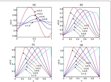
Figure 2Evolution profiles of the numerical solutions with (a)ν= 10–3and (b)ν= 10–6with fixedh= 0.001 andx=10001 for Example1
We solve the problem using fixed time and grid sizes ofh= 0.01 andx=4001 , respec-tively, by varying of the viscosity coefficientsν= 10–k (k= 1, 2, 3, 4) with homogeneous boundary condition. Using the obtained numerical solutions, we calculate the mentioned energyE(t) and massM(t) at discrete time levels and display the results in Fig.1. From the formula of (23),E(t) andM(t) must tend to constants when the viscosity coefficient ν theoretically goes to zero. As expected, the numerical results clearly support that the proposed method has a good performance for both the energy and the mass conservation properties when the viscosity coefficient goes to zero. We additionally observe the behav-iors of the numerical solutions over time for relatively small viscosity coefficientsν= 10–k (k= 3, 6) with homogeneous boundary condition and the results are plotted in Fig.2. In Fig.2, the parameters used in (a)–(b) areh= 0.01,x= 2001 and (c)–(d) areh= 0.002, x=10001 . It can be seen that the proposed method shows good performance even for the advection dominated caseν= 10–6without unnecessary oscillation.
Figure 3Numerical solutions of Example1on the periodic boundary with (a)ν= 10–1, (b)ν= 10–2, (c)ν= 10–3and (d)ν= 10–4
10–4. In other words, asνbecomes smaller, the curves steepen and develop a shock-like
discontinuity. As seen in Fig.3(c) and (d), the proposed method is able to capture the sharp front very well under the periodic boundary conditions. Note that this test is valuable, since the Burgers equation has been studied in a limited work over the periodic boundary conditions compared to non-periodic boundary conditions.
Example2 We consider the two-dimensional unsteady Burgers equation,
ut+uux+uuy=ν(uxx+uyy)
on (x,y)∈[0, 1]2with the Dirichlet boundary condition whose analytic solution [4] is given
by
u(t,x,y) = 1 1 +exp(x+2yν–t).
We first examine the temporal convergence rate for the proposed method for the two vis-cosity coefficientsν= 0.1 andν= 0.01. Results are measured by both the maximum norm and the relativeL2norm errors with a fixed spatial grid sizex=y= 1/2000 and varying
time step sizehat two different timest= 0.1 andt= 1.0. The numerical results are listed in Table1, and they show that the proposed method has second-order temporal conver-gence. Also, to assess the spatial convergence rate for the proposed method,err∞anderrR2
Table 1 Temporal convergence rate for Example2
h t= 0.1 t= 1.0
err∞(t) Rates errR2(t) Rates err∞(t) Rates errR2(t) Rates
ν= 0.1,x=y= 1 2000 1
50 3.23×10
–4 – 2.37×10⁻⁴ – 5.56×10⁻⁴ – 5.01×10⁻⁴ –
1
100 9.00×10
–5 1.84 6.61×10⁻⁵ 1.84 1.44×10⁻⁴ 1.94 1.32×10⁻⁴ 1.92
1
200 2.38×10
–5 1.92 1.74×10⁻⁵ 1.92 3.68×10⁻⁵ 1.97 3.39×10⁻⁵ 1.96
1
400 6.28×10⁻⁶ 1.92 4.39×10⁻⁶ 1.99 9.29×10⁻⁶ 1.99 8.57×10⁻⁶ 1.98 1
800 1.12×10⁻⁶ 2.49 1.28×10⁻⁶ 1.78 2.21×10⁻⁶ 2.07 2.01×10⁻⁶ 2.09
ν= 0.01,x=y=20001 1
50 5.91×10⁻² – 3.29×10⁻² – 3.37×10⁻¹ – 7.08×10⁻² – 1
100 1.17×10⁻² 2.34 8.81×10⁻² 1.90 2.12×10⁻² 3.99 5.18×10⁻³ 3.77 1
200 3.16×10
–3 1.89 2.68×10⁻³ 1.72 3.81×10⁻³ 2.48 1.08×10⁻³ 2.26
1
400 8.54×10
–4 1.89 7.59×10⁻⁴ 1.82 9.46×10⁻⁴ 2.01 2.84×10⁻⁴ 1.93
1
800 2.12×10
–4 2.01 1.90×10⁻⁴ 2.00 2.34×10⁻⁵ 2.02 7.02×10⁻⁵ 2.01
Table 2 Spatial convergence rate for Example2with fixedh= 0.00002
Mx=My t= 0.1 t= 1.0
err∞(t) Rates errR2(t) Rates err∞(t) Rates errR2(t) Rates
ν= 0.1
20 7.45×10⁻⁶ – 7.81×10⁻⁶ – 2.11×10⁻⁵ – 1.30×10⁻⁵ –
40 1.36×10⁻⁷ 5.78 3.28×10⁻⁷ 4.58 1.31×10⁻⁶ 4.02 8.67×10⁻⁷ 3.90
80 1.33×10⁻⁸ 3.36 2.47×10⁻⁸ 3.73 8.16×10⁻⁸ 4.00 5.51×10⁻⁸ 3.98
160 9.59×10⁻¹⁰ 3.79 1.64×10⁻⁹ 3.91 5.24×10⁻⁹ 3.96 3.58×10⁻⁹ 3.94
320 9.00×10⁻¹¹ 3.41 1.67×10⁻¹⁰ 3.30 5.05×10⁻¹⁰ 3.38 3.60×10⁻¹⁰ 3.31
ν= 0.01
40 4.04×10⁻² – 2.16×10⁻² – 2.63×10⁻² – 3.13×10⁻³ –
80 5.90×10⁻⁴ 6.10 3.84×10⁻⁴ 5.81 8.02×10⁻⁴ 5.03 2.07×10⁻⁴ 3.92
160 5.06×10⁻⁵ 3.54 3.00×10⁻⁵ 3.68 5.51×10⁻⁵ 3.86 1.35×10⁻⁵ 3.94
320 3.18×10⁻⁶ 3.99 2.08×10⁻⁶ 3.85 3.39×10⁻⁶ 4.02 8.58×10⁻⁷ 3.98
640 1.98×10⁻⁷ 4.01 1.33×10⁻⁷ 3.96 2.28×10⁻⁷ 3.90 5.99×10⁻⁸ 3.84
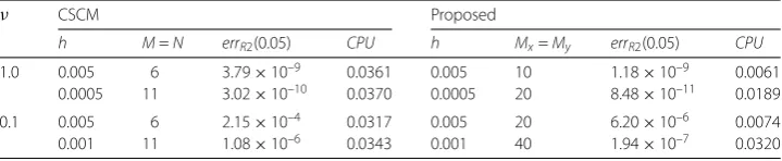
Table 3 Comparison of numerical errors obtained from the proposed method and the CSCM for
Example2
ν CSCM Proposed
h M=N errR2(0.05) CPU h Mx=My errR2(0.05) CPU
1.0 0.005 6 3.79×10⁻⁹ 0.0361 0.005 10 1.18×10⁻⁹ 0.0061
0.0005 11 3.02×10⁻¹⁰ 0.0370 0.0005 20 8.48×10⁻¹¹ 0.0189
0.1 0.005 6 2.15×10⁻⁴ 0.0317 0.005 20 6.20×10⁻⁶ 0.0074
0.001 11 1.08×10⁻⁶ 0.0343 0.001 40 1.94×10⁻⁷ 0.0320
The results are displayed in Table2. It is seen that the rate of spatial convergence is greater than or equal to 3.
To explore the efficiency of the proposed method, the method is compared with the Chebyshev spectral collocation method (CSCM) combined with the fourth-order Runge– Kutta time integration scheme developed by [4]. For the CSCM, we use the numbers of Chebyshev–Gauss–Lobatto pointsNandMshown in Table3. We calculateerrR2at time
result shows that the proposed method is superior to the CSCM in terms of both CPU and accuracy.
Example3 Consider the system of the two-dimensional Burgers equations (8) on (x,y)∈ [0, 1]2with the Dirichlet boundary condition whose analytic solution [4] is given by
u(t,x,y) =v(t,x,y) = 3 4–
1
4(1 +exp(4y–432νx–t)).
We compute the relativeL2 norm error,errR2(t), at two times t= 0.5 andt= 2.0 with
the viscosity coefficientν= 0.01 and fixed spatial grid sizex=y=1601 . Additionally, we investigate the temporal convergence rate by the variation of time step sizes from 1
80
to 25601 . The numerical results are listed in Table4, and the second-order convergence is numerically obtained for the two velocitiesuandv. To explore the efficiency of the present method, we compare the proposed method with the CSCM. The relativeL2 norm error
foruis calculated at timet= 0.01 with various viscosity coefficientsν= 1.0, 0.1, 0.01, and 0.005. The numerical results are displayed in Table5. One can see that our method has a good performance with a significantly reduced computational cost when compared to that of the CSCM. Overall, it could be noted that, with an increased size of the system, there is an increased efficiency in the proposed method when compared to that of the CSCM. It must be noted that the result forvhas a similar aspect to that ofu.
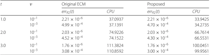
To compare the proposed method and the original ECM in terms of computational costs, we measured the relative L2 norm error and CPU with fixed time and grid sizes
h= 0.005 andx= 1/500 at the different time levelst= 1.0, 2.0 and 3.0, and the results are listed in Table6. Table6shows that the proposed method requires less CPU without any loss in accuracy when compared with the original ECM. Because similar results are obtained forufrom the symmetric property ofuandv, the results ofuare omitted.
Table 4 Temporal convergence rates for Example3, withx=y=1601 andν= 0.01
h t= 0.5 t= 2.0
u v u v
errR2(t) Rates errR2(t) Rates errR2(t) Rates errR2(t) Rates 1
80 2.50×10⁻⁴ – 1.67×10⁻⁴ – 4.28×10⁻⁴ – 2.38×10⁻⁴ – 1
160 1.75×10⁻⁴ 0.51 1.17×10⁻⁴ 0.51 2.38×10⁻⁴ 0.85 1.32×10⁻⁴ 0.85 1
320 9.89×10
–7 7.47 6.61×10⁻⁷ 7.47 8.14×10⁻⁷ 8.19 4.53×10⁻⁷ 8.19
1
640 4.28×10
–7 1.21 2.86×10⁻⁷ 1.21 3.52×10⁻⁷ 1.21 1.96×10⁻⁷ 1.21
1
1280 1.22×10
–7 1.81 8.14×10⁻⁸ 1.81 9.94×10⁻⁸ 1.82 5.53×10⁻⁸ 1.82
1
2560 2.77×10
–8 2.14 1.85×10⁻⁸ 2.14 2.22×10⁻⁸ 2.16 1.24×10⁻⁸ 2.16
Table 5 Comparison of numerical results foruobtained from the proposed method and the CSCM
for Example3
ν CSCM Proposed
h M=N errR2(0.01) CPU h Mx=My errR2(0.01) CPU
1.0 0.0050 11 2.24×10⁻⁶ 0.0956 0.0050 20 3.13×10⁻¹⁵ 0.0063
0.1 0.0025 11 1.87×10⁻⁷ 0.1036 0.0025 20 1.29×10⁻¹⁰ 0.0072
0.01 0.0020 21 7.20×10⁻⁷ 0.1026 0.0020 60 7.31×10⁻⁸ 0.0205
Table 6 Comparison of errors and CPUs ofvvia the proposed method and the original ECM for Example3
t ν Original ECM Proposed
errR2(t) CPU errR2(t) CPU
1.0 10–1 2.21×10⁻⁶ 37.0937 2.21×10⁻⁶ 33.9425
10–3 4.99×10⁻⁴ 37.1391 4.70×10⁻⁴ 34.2735
2.0 10–1 2.03×10⁻⁶ 74.9226 2.03×10⁻⁶ 66.7614
10–3 4.52×10⁻⁴ 74.1522 4.30×10⁻⁴ 66.5531
3.0 10–1 1.76×10⁻⁶ 111.3824 1.76×10⁻⁶ 100.0451
10–3 3.08×10⁻⁴ 110.8592 3.00×10⁻⁴ 99.9561
5 Conclusions
A modified error correction scheme has been developed for efficiently finding numerical solutions in the BSLM framework. Instead of using the traditional way to find the depar-ture points of the particles, we suggest a new technique by constructing new Euler polygon in the error correction strategy, depending on the given boundary conditions. To reduce the computational cost, the proposed method approximates the Jacobian value by a fixed value while maintaining the scale of error, whereas the conventional ECM performs the interpolation with derivatives newly updated in each time integration step. Through sev-eral numerical results, the proposed method has a convergence rate of 2 in time. Also, it is shown that the proposed method obtains outstanding numerical results compared with the existing methods, and it well preserves the energy and mass.
Funding
The first author, Bak, was supported by Basic Science Research Program through the National Research Foundation of Korea (NRF) funded by the Ministry of Education (grant number NRF-2017R1A6A3A01002341). The second author, Kim, the third author, Piao, and the corresponding author, Bu, were supported by the basic science research program through the National Research Foundation of Korea (NRF) funded by the Ministry of Education, Science and Technology (NRF-2016R1A2B2011326, NRF-2017R1C1B1002370 and NRF-2016R1D1A1B03930734), respectively.
Competing interests
The authors declare that they have no competing interests.
Authors’ contributions
All authors jointly worked on the results and they read and approved the final manuscript.
Author details
1Department of Mathematics, Kyungpook National University, Daegu, Republic of Korea.2Department of Liberal Arts,
Hongik University, Sejong, Republic of Korea.
Publisher’s Note
Springer Nature remains neutral with regard to jurisdictional claims in published maps and institutional affiliations.
Received: 30 November 2017 Accepted: 19 November 2018 References
1. Xiu, D., Karniadakis, G.E.: A semi-Lagrangian high-order method for Navier–Stokes equations. J. Comput. Phys.172, 658–684 (2001)
2. Hassanien, I.A., Salama, A.A., Hosham, H.A.: Fourth-order finite difference method for solving Burgers’ equation. Appl. Math. Comput.170, 781–800 (2005)
3. Dehghan, M., Shokri, A.: A numerical method for two-dimensional Schrödinger equation using collocation and radial basis functions. Comput. Math. Appl.54, 136–146 (2007)
4. Khater, A.H., Temsah, R.S., Hassan, M.M.: A Chebyshev spectral collocation method for solving Burgers’-types equations. J. Comput. Appl. Math.222, 333–350 (2008)
5. Liao, W.: An implicit fourth-order compact finite difference scheme for one-dimensional Burgers’ equation. Appl. Math. Comput.206, 755–764 (2008)
7. Wang, J., Layton, A.: New numerical methods for Burgers’ equation based on semi-Lagrangian and modified equation approaches. Appl. Numer. Math.60, 645–657 (2010)
8. Zhang, L., Ouyang, J., Wang, X., Zhang, X.: Variational multiscale element-free Galerkin method for 2D Burgers’ equation. J. Comput. Phys.229, 7147–7161 (2010)
9. Mittal, R.C., Jain, R.K.: Numerical solutions of nonlinear Burgers’ equation with modified cubic B-splines collocation method. Appl. Math. Comput.218, 7839–7855 (2012)
10. Arora, G., Singh, B.K.: Numerical solution of Burgers’ equation with modified cubic B-spline differential quadrature method. Appl. Math. Comput.224, 166–177 (2013)
11. Jiwari, R., Mittal, R.C., Sharma, K.K.: A numerical scheme based on weighted average differential quadrature method for the numerical solution of Burgers’ equation. Appl. Math. Comput.219, 6680–6691 (2013)
12. Zhang, X., Tian, H., Chen, W.: Local method of approximate particular solutions for two-dimensional unsteady Burgers’ equations. Comput. Math. Appl.66, 2425–2432 (2014)
13. Shi, Y., Xu, B., Guo, Y.: Numerical solution of Korteweg–de Vries–Burgers equation by the compact-type CIP method. Adv. Differ. Equ.2015, 353 (2015)
14. Bak, S., Kim, P., Kim, D.: A semi-Lagrangian approach for numerical simulation of coupled Burgers’ equations. Commun. Nonlinear Sci. Numer. Simul.69, 31–44 (2019)
15. Kim, P., Piao, X., Kim, S.D.: An error corrected Euler method for solving stiff problems based on Chebyshev collocation. SIAM J. Numer. Anal.49, 2211–2230 (2011)
16. Kim, S.D., Piao, X., Kim, P.: Convergence on error correction methods for solving initial value problem. J. Comput. Appl. Math.236, 4448–4461 (2012)
17. Piao, X., Bu, S., Bak, S., Kim, P.: An iteration free backward semi-Lagrangian scheme for solving incompressible Navier–Stokes equations. J. Comput. Phys.283, 189–204 (2015)
18. Piao, X., Kim, S., Kim, P., Kwon, J., Yi, D.: An interaction free backward semi-Lagrangian scheme for guiding center problem. SIAM J. Numer. Anal.53, 619–643 (2015)
19. Ewing, R.E., Wang, H.: A summary of numerical methods for time-dependent advection-dominated partial differential equations. J. Comput. Appl. Math.128, 423–445 (2001)
20. Fornberg, B.: Calculation of weights in finite difference formulas. SIAM Rev.40, 685–691 (1998) 21. Evans, C.L.: Partial Differential Equations. Am. Math. Soc., Providence (1998)
22. Ladyzenskaya, O.A., Solnnikov, V.A., Ura´lceva, N.N.: Linear and Quasilinear Equations of Parabolic Type. Am. Math. Soc., Providence (1968)
23. Kim, D., Song, O., Ko, H.-S.: A semi-Lagrangian CIP fluid solver without dimensional splitting. Comput. Graph. Forum
27, 467–475 (2008)