R E S E A R C H
Open Access
Hybrid variational model based on
alternating direction method for
image restoration
Jianguang Zhu
1, Kai Li
1and Binbin Hao
2**Correspondence: [email protected]
2College of Science, China University of Petroleum, Qingdao, P.R. China
Full list of author information is available at the end of the article
Abstract
The total variation model is widely used in image deblurring and denoising process with the features of protecting the image edge. However, this model usually causes some staircase effects. To overcome the shortcoming, combining the second-order total variation regularization and the total variation regularization, we propose a hybrid total variation model. The new improved model not only eliminates the staircase effect, but also well protects the edges of the image. The alternating direction method of multipliers (ADMM) is employed to solve the proposed model. Numerical results show that our proposed model can get more details and higher image visual quality than some current state-of-the-art methods.
Keywords: Total variation; Image restoration; Staircase effect; Alternating direction method of multipliers
1 Introduction
Image restoration mainly includes image deblurring and image denoising, which is one of the most fundamental problems in imaging science. It plays an important role in many mid-level and high-level image-processing areas such as medical imaging, remote sensing, machine identification, and astronomy [1–4]. The image restoration problem usually can be expressed in the following form:
g=Hf+η, (1.1)
wheref ∈Rn2is the originaln×nimage,H∈Rn2×n2 is a blurring operator,η∈Rn2is the white Gaussian noise, andg∈Rn2is a degraded image.
It is well known that the image restoration problem is usually an ill-posed problem. An efficient method to overcome the ill-posed problems is to add some regularization terms to the objective functions, which is known as a regularization method. There are two fa-mous regularization methods. One is the Tikhonov regularization [5], and the other is the total variation (TV) regularization [6]. The Tikhonov regularization method has a disad-vantage, which tends to make images overly smooth and often fails to adequately preserve important image attributes such as sharp edges. The total variation regularization method has the ability to preserve edges well and remove noise at the same time, which was first
introduced by Rudin et al. [6] as follows:
min
f Hf –g 2
2+αfTV, (1.2)
where · 2denotes the Euclidean norm, · TVis the discrete total variation regulariza-tion term, andαis a positive regularization parameter that controls the tradeoff between these two terms. To define the discrete TV norm, we first introduce the discrete gradient
∇f:
Due to the nonlinearity and nondifferentiability of the total variation function, it is dif-ficult to solve model (1.2). To solve this problem more effectively, many methods have been proposed for total-variation-based image restoration in recent years [6–27]. In these methods, Rudin et al. [6] raised a time marching scheme, and Vogel et al. [7] put forward a fixed point iteration method. The time marching scheme converges slowly, especially when the iterate point is close to the solution set. The fixed point iteration method is also very difficult to solve as the blurring kernel becomes larger. Based on the dual formulation, Chambolle [15] proposed a gradient algorithm for the total variation denoising problem. At present, based on variable separation and penalty techniques, Wang et al. [16] proposed the fast total variant deconvolution (FTVd) method. By introducing an auxiliary variable to replace the nondifferentiable part of model (1.2), the TV model (1.2) can be rewritten in the following minimization problem:
whereβis a penalty parameter. Experimental results verify the effectiveness of the FTVd method. But in the calculation, the penalty parameterβneeds to approach infinity, which creates numerical instability. To avoid the approach of penalty parameter to infinity, Chan et al. [28] proposed the alternating direction method of multipliers (ADMM) to solve model (1.2). By defining the augmented Lagrange function, the image restoration model (1.2) can be translated into the following form:
whereλis a Lagrange multiplier. The experimental results show that the ADMM method is robust and fast, and has a good restoration effect.
More recently, to overcome the shortcoming of the TV norm off in model (1.2), Huang et al. [29] proposed a fast total variation minimization method for image restoration as follows:
min
f,u Hf –g 2
2+α1f–u22+α2uTV, (1.3) where α1,α2 are positive regularization parameters. Model (1.3) adds a termf –u22, compared with model (1.2). The experimental results show that the modified TV mini-mization model can preserve edges very well in the image restoration processing. Based on model (1.3), Liu et al. [30] proposed the following minimization model:
min
f,u Hf –g 2
2+α1f–u22+α2fTV+α3uTV, (1.4) whereα1,α2, andα3are positive regularization parameters. Liu et al. [30] adopted the split Bregman method and Chambolle projection algorithm to solve the minimization model (1.4). Numerical results illustrated the effectiveness of their model.
Although the total variation regularization can preserve sharp edges very well, it also causes some staircase effects [31,32]. To overcome this kind of staircase effect, some high-order total variational models [33–39] and fractional-order total variation models [40–44] are introduced. It has been proved that the high-order TV norm can remove the staircase effect and preserve the edges well in the process of image restoration.
To eliminate the staircase effect better and preserve edges very well in image process-ing, we combine the TV norm and second-order TV norm and introduce a new hybrid variational model as follows:
min
f,u Hf –g 2
2+α1f–u22+α2∇2f2+α3∇u2, (1.5) whereα1,α2, andα3are positive regularization parameters,∇u2is the TV norm ofu, and∇2f
2 is the second-order TV norm of f. The definition of the second-order TV norm is similar to that of the TV norm. The second-order TV norm is defined by
∇2f
i,j=
(∇f)x,xi,j, (∇f)x,yi,j, (∇f)y,xi,j, (∇f)y,yi,j,
∇2f= 1≤i,j≤n
(∇f)x,xi,j 2+ (∇f)x,yi,j 2+ (∇f)y,xi,j 2+ (∇f)y,yi,j 2,
where (∇f)x,xi,j, (∇f)x,yi,j, (∇f)y,xi,j, (∇f)y,yi,j denote the second-order differences of the ((j– 1)n+i)th entry of the vectorf. For more detail about the second-order differences, we refer to [45]. The second-order TV regularization and TV regularization are used; the edges in the restored image can be preserved quite well, and the staircase effect is reduced simultaneously.
2 The alternating iterative algorithm
In this section, we use an alternating iterative algorithm to solve (1.5). Based on the vari-able separation technique [16], the minimization problem (1.5) can be divided into de-blurring and denoising steps. The alternating iterative algorithm is based on decoupling of denoising and deblurring steps in the image restoration process. The deblurring step is defined as
arg min
f Hf–g 2
2+α1f –u22+α2∇2f2. (2.1) The denoising step is defined as
arg min
u α1u–f 2
2+α3∇u2. (2.2)
We adopt the alternating direction multiplier method to solve these two subproblems.
2.1 The deblurring step
Because the ADMM method has the characteristics of notable stability and high rate of convergence, this method can avoid the approach of penalty parameter to infinity. We employ the alternating direction method of multipliers to solve the minimization prob-lem (2.1). Because the objective function of (2.1) is nondifferentiable, by introducing an auxiliary variableω, the unconstrained optimization problem (2.1) can be transformed into the following equivalent constraint optimization problem:
arg min
f,ω Hf–g 2
2+α1f –u22+α2ω2 s.t.ω=∇2f. (2.3) For the constrained optimization problem (2.3), its augmented Lagrange function is de-fined by
where λ1 is a Lagrange multiplier, playing the role of avoiding the positive penalty pa-rameters to go to infinity, and β1 is a positive penalty parameter. Then, the alternating minimization method to minimize problem (2.4) can be expressed as follows:
Based on the optimal conditions, the solution of (2.6) is given by the equation
where∇2T is the conjugate operator of∇2. Under the periodic boundary condition,HTH and∇2T∇2are block circulant matrices [46,47], soHTHand∇2T∇2can be diagonalized by the Fourier transform. The Fourier transform off is denoted byF(f), andF–1(f) is the inverse Fourier transform off. By using the Fourier transform the solution off can be given as follows:
The subproblem forωcan be written as
ωk+1=arg min
and the solution can be explicitly obtained using the following two-dimensional shrinkage operator [16,48]:
where we follow the convention that 0·(0/0) = 0. Finally, we updateλ1by
λk+11 =λk1+ηβ1
ωk+1–∇2fk+1, (2.11)
whereηis a relaxation parameter, andη∈(0, (√5 + 1)/2).
The algorithm of the deblurring step is summarized in Algorithm1.
2.2 The denoising step
Subproblem (2.2) is a classical TV regularization process for image denoising, which can be solved by the Chambolle projection algorithm. However, it is well known that the Chambolle projection algorithm has large amount of calculations in the process of ex-periment and causes numerical instability. To overcome the disadvantage of numerical instability and large amount of calculations of the Chambolle projection algorithm, in this paper, we adopt the alternating direction multiplier method to solve subproblem (2.2).
Algorithm 1Alternating direction minimization method for solving subproblem (2.1)
Second, to use the alternating direction multiplier method to solve model (2.12), we define its augmented Lagrangian function
whereβ2is a positive penalty parameters, andλ2is a Lagrange multiplier.
The variablesu,f,vare coupled together, so we separate this problem into two subprob-lems and adopt the alternating iteration minimization method. The two subprobsubprob-lems are given as follows.
The “u-subproblem” forvfixed:
min
The “v-subproblem” forufixed:
min
The minimizer of subproblem (2.14) can be simplified as
min
and the minimization problem (2.16) can be solved by the following equation:
2α1I+β2∇T∇
Algorithm 2Alternating direction minimization method for solving the subproblem (2.2)
Next, the minimization of (2.15) with respect to vis equivalent to the minimization problem
and the solution of (2.18) can be explicitly obtained by the two-dimensional shrinkage:
vk+1=max∇uk+1–λ
The Lagrange multiplierλ2is updated as follows:
λk+12 =λk2+ηβ2
vk+1–∇uk+1, (2.20)
whereηis a relaxation parameter.
The algorithm of the denoising step is written in Algorithm2.
3 Numerical experiments
This section presents some numerical examples, which show that the performance of our proposed algorithm to solve image restoration problems. In the following experiments, we compare our proposed method (HTV) with Fast-TV [29] and FNDTV methods [30]. All experiments are performed under Windows 7 and MATLAB 2012a running on a desktop with an core i5 Duo central processing unit at 2.50 GHz and 4 GB memory. The quality of the restoration results by different methods is compared quantitatively by using the peak-signal-to-noise ratio (PSNR) and structural similarity index metric (SSIM). Supposeg,f0, anduare the observed image, the ideal image, and the restored image, respectively. Then, the BSNR, MSE, PSNR, and SSIM are defined as follows:
PSNR = 20log10MAX√ f0
MSE,
SSIM = (2μf0μu+c1)(2σf0u+c2) (μ2f0+μ2u+c1)(σf20+σu2+c2)
,
whereηis the additive noise vector,n2is the number of pixels of image, MAX f0 is the
maximum possible pixel value of the f0, f¯ is the mean intensity value off0, μ f0 is the
mean value of thef0,μuis the mean value ofu,σf20 andσu2are the variances off0andu, respectively, andσf0uis the covariance off0andu, andc1andc2are stabilizing constants
for near-zero denominator values. We will also use the SSIM index map to reveals areas of high/low similarity between two images; the whiter the SSIM index map, the closer the two images. Further details on SSIM can be founded in the pioneer work [49].
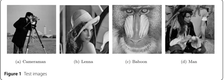
Four test images, “Cameraman”, “Lena”, “Baboon”, and “Man”, which are commonly used in the literature, are shown in Fig.1. We test three kinds of blur, that is, Gaussian blur, average blur, and motion blur. These different blurring kernels can be builded by the func-tion “fspecial” in the Matlab. The additive noise is a Gaussian noise in all experiments. In all tests, we add the Gaussian white noise of different BSNR to the blurred images. In our experiments, the stopping criterion is that the relative difference between the successive iteration of the restored image should satisfy the inequality
fk+1–fk 2
fk
2 ≤
1×10⁻⁴,
wherefkis the computed image at thekth iteration of the tested method. In the following experiments, for our proposed method, we fixed the parameterα2= 1.3e–2 for all exper-iments,α1= 1e–4 (for Gaussian blur and average blur), 3e–4 (for motion blur),α3= 1e–4 (for Gaussian blur and average blur), 2e–4 (for motion blur). For the parameters of FastTV and FNDTV, we refer to [29,30]. The parameters for every compared method are selected from many experiments until we obtain the best PSNR values.
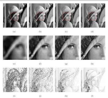
Figure2shows the experiment for Gaussian blur. We select the “Cameraman” image (256×256) as the test image, which is shown in Figure1(a). The “Cameraman” image de-graded by Gaussian blur with blur nucleus 9∗9 and a noise with BSNR = 35 is shown in Fig.2(a). The recovered images by FastTV, FNDTV, and our method are shown in Fig.2(b)–(d). To demonstrate the effectiveness of our method more intuitively, we en-large some part of the three restored images, and the results of enen-larged parts are shown in Fig.2(e)–(h). We also show the SSIM index maps of the restored images recovered by
Figure 2Results of different methods when restoring blurred and noisy image “Cameraman” degraded by Gaussian blur with Gaussian blur nucleus 9∗9 and a noise withBSNR= 35: (a) blurred and noisy image; (b) restored image by FastTV; (c) restored image by FNDTV; (d) restored image by our method; (e) zoomed part of (a); (f) zoomed part of (b); (g) zoomed part of (c); (h) zoomed part of (d); (i) SSIM index map of the corrupted image; (j) SSIM index map of the recovered image by FastTV; (k) SSIM index map of the recovered image by FNDTV; (l) SSIM index map of the recovered image by our method
the three methods in Fig.2(i)–(l). The SSIM map of the restored image by the proposed method is slightly whiter than the SSIM map by FastTV and FNDTV. The values of PSNR and SSIM by these methods are shown in Table1. We see that both PSNR and SSIM val-ues of the restored image by our proposed method are higher than FastTV and FNDTV. We also plot the changing curve of SSIM versus iterations with three different methods in Fig.3. It is not difficult to see that our method can achieve a high SSIM over the other two methods with a few iterations. In addition, for the restoration effect of other images, we depict them by PSNRs and SSIMs; see Table1. It is easy to detect that both of PSNR and SSIM of the restored image by our method are higher than others obtained by FastTV and FNDTV.
meth-Table 1 Experimental results for different images and different blur kernels,BSNR= 35
Image Blur kernels Fast-TV [26] FNDTV [27] Our
PSNR SSIM PSNR SSIM PSNR SSIM
Cameraman Gaussian(5, 5) 27.0656 0.4399 27.2341 0.4417 27.8678 0.4562
Gaussian(7, 7) 26.1232 0.3992 26.8021 0.4155 27.0689 0.4383
Gaussian(9, 9) 24.9719 0.3807 25.6502 0.4024 26.4150 0.4057
Couple Gaussian(5, 5) 31.3219 0.7337 31.6776 0.7595 32.8470 0.7889
Gaussian(7, 7) 29.9460 0.6767 30.7103 0.6989 31.3003 0.7321
Gaussian(9, 9) 29.2731 0.6694 29.8778 0.6739 30.6027 0.6963
Lenna average(7) 31.3460 0.6673 31.8335 0.6916 32.6287 0.7256
average(9) 30.5242 0.6415 31.0531 0.6541 31.6273 0.6737
average(11) 29.5574 0.6134 30.4395 0.6376 30.9392 0.6481
Goldhill average(7) 28.3139 0.6077 29.2712 0.6188 30.0464 0.6330
average(9) 28.1314 0.5816 28.3268 0.5990 28.5740 0.6023
average(11) 26.8336 0.5244 27.4211 0.5576 27.8857 0.5744
Man motion(20, 20) 29.8667 0.6258 30.1235 0.6622 30.8716 0.6864
motion(10, 100) 30.5363 0.6839 31.2202 0.7130 32.5163 0.7314
Baboon motion(20, 20) 27.4672 0.7968 27.8722 0.8334 28.5560 0.8508
motion(10, 100) 28.8783 0.8213 28.9383 0.8621 29.3343 0.8778
Figure 3Changes of SSIM value versus iteration number for the three methods about Gaussian blur
ods is shown in Fig. 4(i)–(l). It is easy to see that the SSIM map obtained by the pro-posed method is slightly whiter than the maps by the other two methods. In Fig.5, we plot the changes of SSIM value versus iteration number for the three methods. It can also be found from the relationship between SSIM values and iteration numbers that our method requires fewer iterations and the values are superior to the other two methods. These experiments demonstrate the outstanding performance of our proposed method to over-come the blocky images while preserving edge details. We also report the PSNR and SSIM values by these methods in Table1. The PSNR and SSIM values of the restored image by our proposed method are higher than those of FastTV and FNDTV.
Figure 4Results of different methods when restoring blurred and noisy image “Lenna” degraded by average blur with length 9 and a noise withBSNR= 35: (a) blurred and noisy image; (b) restored image by Fast-TV; (c) restored image by FNDTV; (d) restored image by our method; (e) zoomed part of (a); (f) zoomed part of (b); (g) zoomed part of (c); (h) zoomed part of (d); (i) SSIM index map of the corrupted image; (j) SSIM index map of the recovered image by FastTV; (k) SSIM index map of the recovered image by FNDTV; (l) SSIM index map of the recovered image by our method
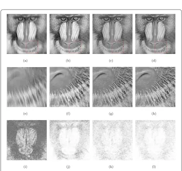
Figure 6Results of different methods when restoring blurred and noisy image “Man” degraded by motion blur withlen= 20 andtheta= 20 and a noise withBSNR= 35: (a) blurred and noisy image; (b) restored image by Fast-TV; (c) restored image by FNDTV; (d) restored image by our method; (e) zoomed part of (a); (f) zoomed part of (b); (g) zoomed part of (c); (h) zoomed part of (d); (i) SSIM index map of the corrupted image; (j) SSIM index map of the recovered image by FastTV; (k) SSIM index map of the recovered image by FNDTV; (l) SSIM index map of the recovered image by our method
(h). We also show the SSIM index maps of the restored images recovered by the three methods in Figs.6and8(j)–(l). It is easy to see that the SSIM map of the restored image by the proposed method is slightly whiter than the SSIM map by FastTV and FNDTV. In Figs.7and9, we plot the changes of SSIMs with iteration number for FastTV method, FNDTV method, and our method. From Figs.7and9, we can see that our method can get higher image visual quality and more details than Fast-TV method and FNDTV method. The values of PSNR and SSIM are listed in Tables1and2. We see that both the PSNR and SSIM values of the restored image by the proposed method are much better than those provided by FastTV and FNDTV.
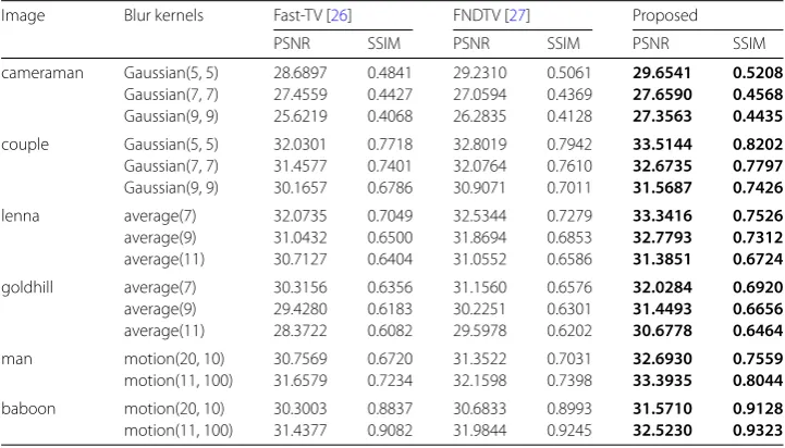
The numerical results of three different methods in terms of PSNR and SSIM are shown in the following tables. From Tables1and2it is not difficult to see that the PSNR and SSIM of the restored image by our proposed method are higher than those obtained by FastTV and FNDTV.
4 Conclusion
Figure 7Changes of SSIM value versus iteration number for the three methods about motion blur with
theta= 20
Figure 9Changes of SSIM value versus iteration number for the three methods about motion blur with
theta= 100
Table 2 Experimental results for different images and different blur kernels,BSNR= 40
Image Blur kernels Fast-TV [26] FNDTV [27] Proposed
PSNR SSIM PSNR SSIM PSNR SSIM
cameraman Gaussian(5, 5) 28.6897 0.4841 29.2310 0.5061 29.6541 0.5208
Gaussian(7, 7) 27.4559 0.4427 27.0594 0.4369 27.6590 0.4568
Gaussian(9, 9) 25.6219 0.4068 26.2835 0.4128 27.3563 0.4435
couple Gaussian(5, 5) 32.0301 0.7718 32.8019 0.7942 33.5144 0.8202
Gaussian(7, 7) 31.4577 0.7401 32.0764 0.7610 32.6735 0.7797
Gaussian(9, 9) 30.1657 0.6786 30.9071 0.7011 31.5687 0.7426
lenna average(7) 32.0735 0.7049 32.5344 0.7279 33.3416 0.7526
average(9) 31.0432 0.6500 31.8694 0.6853 32.7793 0.7312
average(11) 30.7127 0.6404 31.0552 0.6586 31.3851 0.6724
goldhill average(7) 30.3156 0.6356 31.1560 0.6576 32.0284 0.6920
average(9) 29.4280 0.6183 30.2251 0.6301 31.4493 0.6656
average(11) 28.3722 0.6082 29.5978 0.6202 30.6778 0.6464
man motion(20, 10) 30.7569 0.6720 31.3522 0.7031 32.6930 0.7559
motion(11, 100) 31.6579 0.7234 32.1598 0.7398 33.3935 0.8044
baboon motion(20, 10) 30.3003 0.8837 30.6833 0.8993 31.5710 0.9128
motion(11, 100) 31.4377 0.9082 31.9844 0.9245 32.5230 0.9323
the proposed model can obtain better results than those restored by some existing restora-tion methods. It also shows that the new model can obtain a better visual resolurestora-tion than the other two methods.
Acknowledgements
The authors would like to thank the referees for their valuable comments and suggestions.
Funding
This work was supported by National Key Research and Development Program of China (No. 2017YFC1405600), by the Training Program of the Major Research Plan of National Science Foundation of China (No. 91746104), by National Science Foundation of China (Nos. 61101208, 11326186), Qindao Postdoctoral Science Foudation (No. 2016114), Project of Shandong Province Higher Educational Science and Technology Program (No. J17KA166), Joint Innovative Center for Safe and Effective Mining Technology and Equipment of Coal Resources, Shandong Province of China and SDUST Research Fund (No. 2014TDJH102).
Competing interests
The authors declare that there is no conflict of interest regarding the publication of this paper.
Authors’ contributions
Author details
1College of Mathematics and Systems Science, Shandong University of Science and Technology, Qingdao, P.R. China. 2College of Science, China University of Petroleum, Qingdao, P.R. China.
Publisher’s Note
Springer Nature remains neutral with regard to jurisdictional claims in published maps and institutional affiliations.
Received: 23 March 2018 Accepted: 2 December 2018
References
1. Hajime, T., Hayashi, T., Nishi, T.: Application of digital image analysis to pattern formation in polymer systems. J. Appl. Phys.59(11), 3627–3643 (1986)
2. Chen, M., Xia, D., Han, J., Liu, Z.: An analytical method for reducing metal artifacts in X-ray CT images. Math. Probl. Eng. 2019, Article ID 2351878 (2019)
3. Chen, M., Li, G.: Forming mechanism and correction of CT image artifacts caused by the errors of three system parameters. J. Appl. Math.2013, Article ID 545147 (2013)
4. Chen, Y., Guo, Y., Wang, Y., et al.: Denoising of hyperspectral images using nonconvex low rank matrix approximation. IEEE Trans. Geosci. Remote Sens.55(9), 5366–5380 (2017)
5. Tikhonov, A.N., Arsenn, V.Y.: Solution of Ill-Posed Problem. Winston and Sons, Washington (1977)
6. Rudin, L.I., Osher, S., Fatemi, E.: Nonlinear total variation based noise removal algorithms. Physics D60, 259–268 (1992) 7. Vogel, C.R., Oman, M.E.: Iterative methods for total variation denoising. SIAM J. Sci. Comput.17, 227–238 (1996) 8. Zhu, J.G., Hao, B.B.: A new noninterior continuation method for solving a system of equalities and inequalities. J. Appl.
Math.2014, Article ID 592540 (2014)
9. Yu, J., Li, M., Wang, Y., He, G.: A decomposition method for large-scale box constrained optimization. Appl. Math. Comput.231(12), 9–15 (2014)
10. Han, C., Feng, T., He, G., Guo, T.: Parallel variable distribution algorithm for constrained optimization with nonmonotone technique. J. Appl. Math.2013, Article ID 295147 (2013)
11. Sun, L., He, G., Wang, Y.: An accurate active set newton algorithm for large scale bound constrained optimization. Appl. Math.56(3), 297–314 (2011)
12. Zheng, F., Han, C., Wang, Y.: Parallel SSLE algorithm for large scale constrained optimization. Appl. Math. Comput. 217(12), 5277–5384 (2011)
13. Zhu, J., Hao, B.: A new smoothing method for solving nonlinear complementarity problems. Open Math.17(1), 21–38 (2019)
14. Tian, Z., Tian, M., Gu, C.: An accelerated jacobi gradient based iterative algorithm for solving sylvester matrix equations. Filomat31(8), 2381–2390 (2017)
15. Chambolle, A.: An algorithm for total variation minimization and applications. J. Math. Imaging Vis.20(1–2), 89–97 (2004)
16. Wang, Y., Yang, J., Yin, W., et al.: A new alternating minimization algorithm for total variation image reconstruction. SIAM J. Imaging Sci.1(3), 248–272 (2008)
17. Zhang, R.Y., Xu, F.F., Huang, J.C.: Reconstructing local volatility using total variation. Acta Math. Sin. Engl. Ser.33(2), 263–277 (2017)
18. Bai, Z.B., Dong, X.Y., Yin, C.: Existence results for impulsive nonlinear fractional differential equation with mixed boundary conditions. Bound. Value Probl.2016, 63 (2016)
19. Wang, Z.: A numerical method for delayed fractional-order differential equations. J. Appl. Math.2013, 256071 (2013) 20. Wang, Z., Huang, X., Zhou, J.P.: A numerical method for delayed fractional-order differential equations: based on G-L
definition. Appl. Math. Inf. Sci.7(2), 525–529 (2013)
21. Zhang, Y.L., Lv, K.B., et al..: Modeling gene networks in Saccharomyces cerevisiae based on gene expression profiles. Comput. Math. Methods Med.2015, Article ID 621264 (2015)
22. Lu, X., Wang, H.X., Wang, X.: On Kalman smoothing for wireless sensor networks systems with multiplicative noises. J. Appl. Math.2012, 203–222 (2012)
23. Ding, S.F., Huang, H.J., Xu, X.Z., et al.: Polynomial smooth twin support vector machines. Appl. Math. Inf. Sci.8(4), 2063–2071 (2014)
24. Goldfarb, D., Yin, W.: Second-order cone programming methods for total variation based image restoration. SIAM J. Sci. Comput.27(2), 622–645 (2005)
25. Han, C.Y., Zheng, F.Y., Guo, T.D., He, G.P.: Parallel algorithms for large-scale linearly constrained minimization problem. Acta Math. Appl. Sin. Engl. Ser.30(3), 707–720 (2014)
26. Hao, B.B., Zhu, J.G.: Fast L1 regularized iterative forward backward splitting with adaptive parameter selection for image restoration. J. Vis. Commun. Image Represent.44, 139–147 (2017)
27. Morini, B., Porcelli, M., Chan, R.H.: A reduced Newton method for constrained linear least squares problems. J. Comput. Appl. Math.233, 2200–2212 (2010)
28. Chan, R.H., Tao, M., Yuan, X.: Constrained total variation deblurring models and fast algorithms based on alternating direction method of multipliers. SIAM J. Imaging Sci.6(1), 680–697 (2013)
29. Huang, Y.M., Ng, M.K., Wen, Y.W.: A fast total variation minimization method for image restoration. Multiscale Model. Simul.7(2), 774–795 (2008)
30. Liu, J., Huang, T.Z., et al..: An efficient variational method for image restoration. Abstr. Appl. Anal.2013, 213536 (2013) 31. Chambolle, A., Lions, P.L.: Image recovery via total variation minimization and related problems. Numer. Math.76,
167–188 (1997)
32. Chan, T., Marquina, A., Mulet, P.: High-order total variation-based image restoration. SIAM J. Sci. Comput.22(2), 503–516 (2000)
34. Liu, G., Huang, T., Liu, J.: High-order TVL1-based images restoration and spatially adapted regularization parameter selection. Comput. Math. Appl.67, 2015–2026 (2014)
35. Zhu, G.J., Li, K., Hao, B.B.: Image restoration by a mixed high-order total variation and l1 regularization model. Math. Probl. Eng.2018, Article ID 6538610 (2018)
36. Lysaker, M., Tai, X.C.: Iterative image restoration combining total variation minimization and a second-order functional. Int. J. Comput. Vis.66(1), 5–18 (2006)
37. Zhu, J., Liu, K., Hao, B.: Restoration of remote sensing images based on nonconvex constrained high-order total variation regularization. J. Appl. Remote Sens.13(2), 022006 (2019)
38. You, Y.L., Kaveh, M.: Fourth-order partial differential equations for noise removal. IEEE Trans. Image Process.9(10), 1723–1730 (2000)
39. Hajiaboli, M.R.: An anisotropic fourth-order diffusion filter for image noise removal. Int. J. Comput. Vis.92(2), 177–191 (2011)
40. Chen, D., Chen, Y., Xue, D.: Fractional-order total variation image denoising based on proximity algorithm. Appl. Math. Comput.257, 537–545 (2015)
41. Wang, Z., Xie, Y., Lu, J.,et al..: Stability and bifurcation of a delayed generalized fractional-order prey–predator model with interspecific competition. Appl. Math. Compt.347, 360–369 (2019)
42. Wang, X., Wang, Z., Huang, X.,et al..: Dynamic analysis of a fractional-order delayed SIR model with saturated incidence and treatment functions. Int. J. Bifurcat. Chaos28(14), 1850180 (2018)
43. Jiang, C., Zhang, F., Li, T.: Synchronization and antisynchronization of N-coupled fractional-order complex systems with ring connection. Math. Methods Appl. Sci.41(3), 2625–2638 (2018)
44. Ren, Z., He, C., Zhang, Q.: Fractional order total variation regularization for image super-resolution. Signal Process. 93(9), 2408–2421 (2013)
45. Wu, C., Tai, X.C.: Augmented Lagrangian method, dual methods, and split Bregman iteration for ROF, vectorial TV, and high order models. SIAM J. Imaging Sci.3(3), 300–339 (2010)
46. Michael, N., Chan, R.H., Tang, W.C.: A fast algorithm for deblurring models with Neumann boundary conditions. SIAM J. Sci. Comput.21(3), 851–866 (1999)
47. Gonzalez, R.C., Woods, R.E.: Digital Image Processing, 3rd edn. Prentice Hall, New York (2011)
48. Yang, J.F., et al.: A fast algorithm for edge-preserving variational multichannel image restoration. SIAM J. Imaging Sci. 2, 569–592 (2011)