The classification of the single traveling wave solutions to \((1+1)\) dimensional Gardner equation with variable coefficients

(1)

R E S E A R C H

Open Access

The classiﬁcation of the single traveling

wave solutions to

(1 + 1)

dimensional

Gardner equation with variable coefﬁcients

Damin Cao

1*

_{and Lijuan Du}

1

*_{Correspondence:} [email protected] 1_{School of Air Transportation,}

Shanghai University of Engineering Science, Shanghai, P.R. China

Abstract

In this paper the classification of single traveling wave solutions of (1 + 1) dimensional Gardner equation with variable coefficients is obtained by applying the complete discrimination system to the polynomial and trial equation methods. In particular, the corresponding solutions for the concrete parameters are constructed to show that each solution in the classification can be realized. Moreover, numerical simulations shown in the paper could help us better understand the nature of each solution.

Keywords: Exact solution; (1 + 1) dimensional Gardner equation with variable

coeﬃcients; Complete discrimination system for polynomial method; Trial equation method; Traveling wave solutions

1 Introduction

Nonlinear differential equations have been widely applied to describe physical phenom-ena in many scientific fields, such as physics, electronics and other engineering and applied sciences. For hundreds of years, scientists have been studying both the exact and numer-ical solutions of nonlinear problems [1–4]. Due to the inaccuracy of numerical solutions, especially when we encounter very sensitive problems such as chaos, exact solutions have important applications. Accurate solutions can also help us better understand physical phenomena and models. Therefore, finding the exact solutions is of great significance.

A shallow water wave (or long wave) is considered a nonlinear dynamic system with wavelength much longer than its depth. It is widely used to describe nonlinear phenom-ena in the atmosphere and ocean. In order to describe and study the related nonlinear problems, the KdV equation [5] has been established. However, in some situations, the modified KdV equation should be applied when we discuss the effect of surface tension. But in some conditions such as internal solitary waves in a two-layer fluid with surface ten-sion where the KdV and mKdV equation are not valid at some thickness ratios, we need to combine the KdV equation and mKdV, namely study the Gardner equation, which takes the surface tension on solitary waves in a two-layer (stratified) fluid [6] into consideration. The one-dimensional variable-coefficient Gardner equation

ut+a(t)ux+b(t)u2ux+c(t)uxxx= 0, (1)

(2)

wherea(t),b(t),c(t) are nonzero arbitrary functions, was proposed to describe internal solitary waves that occur in coastal areas with inhomogeneous media and boundary, such as the northwest continental shelf of Australia and the Baltic Sea [7, 8]. In this paper, the trial equation method [9–14] and the complete discrimination system for polynomial method [15–20] are applied to the generalized (1 + 1) dimensional Gardner equation with variable coeﬃcients. In order to ensure the existence of the solutions, the concrete exam-ples of speciﬁc parameters are given.

In real life applications, most nonlinear differential equations (or systems of differential equations) contain arbitrary functions of dependent variables and their derivatives. Ex-tensive studies have been conducted by using various numerical and analytical methods for the various forms of equations that emerge. However, these approaches may involve approximate solutions [21]. In recent years, many useful methods have been put forward, such as direct method [22], improved tanh–coth method [23], and so on. However, few methods can get all the traveling wave solutions to the nonlinear equations. So Liu pro-posed the trial equation method and the complete discrimination system for polynomial method. By these two methods, many difficult problems have been solved [24]. According to [10], we can see that, by taking a special traveling wave transformation

u(x,y, . . . ,t) =φ(ξ), ξ=κ1(t)x+κ2(t)y+· · ·+ω(t), (2)

we can actually reduce the nonlinear diﬀerential equation with variable coeﬃcients

Ψ(t,x,y,u,ux,uy, . . . ) = 0, (3)

to the nonlinear ordinary equation

ψt,x,y,k1,k2,ωu,u,u, . . .= 0. (4)

Then, by taking the following trial equation:

u2=F(u), (5)

and substituting Eq. (5) into Eq. (4), an ordinary equation system is obtained, and the trial functionF(u) could be a polynomial, rational function, or some other irrational function. Upon getting the trial equation, we can obtain the integral form of the original equation as

±(ξ–ξ0) =

dφ

G(φ), (6)

(3)

2 The classiﬁcation of traveling wave solutions to(1 + 1)dimensional Gardner equation with variable coefﬁcients

To find the classification of traveling wave solutions to (1 + 1) dimensional Gardner equa-tion with variable coefficients, we set

u(x,t) =φ(ξ), ξ=κ(t)x+ω(t), (7)

whereκ(t),ω(t) represent nonzero arbitrary functions. Substituting Eq. (7) into Eq. (1) yields

κ(t)x+ω(t)φ+a(t)κ(t)φφ+b(t)κ(t)φ2φ+c(t)κ3(t)φ= 0. (8)

Now we assume that (φ)2is equal to a polynomial function, namely

φ2=anφn+an–1φn–1+· · ·+a1φ+a0, (9)

and, via the balance principle, we getn= 4, so

φ2=a4φ4+a3φ3+a2φ2+a1φ+a0. (10)

Then taking derivatives on both sides of Eq. (10), we have

φ= 6a4φ2φ+ 3a3φφ+a2φ. (11)

Substituting (11) into (8), we get

dκ(t)

dt x+

dω(t)

dt +a2c(t)κ

3₍_t_{) = 0,} ₍₁₂₎

a(t)κ(t) + 3a3c(t)κ3(t) = 0, (13)

b(t)κ(t) + 6a4c(t)κ3(t) = 0. (14)

Actually, this system of equations is not solvable. So we must impose some restrictions on it. Settinga3= 2b1a4, whereb1is a constant, we have

a(t) =b1b(t), (15)

dκ(t)

dt x= 0, (16)

dω(t)

dt = –

b(t)κ(t) 6a4

. (17)

So we getκ(t) =const, and by settingκ(t) =κ, we obtain

ω(t) = –

κb(t)

6a4

dt. (18)

Let

Φ= (a4)

1 4

φ+b1

2

, ξ1= (a4)

1

(4)

then Eq. (10) is deformed into

Then the corresponding complete discrimination system is presented as [11]

D1= 4, D2= –p, D3= –2p3+ 8pr– 9q2, E2= 9q2– 32pr,

D4= –p3q2+ 4p4r+ 36pq2– 32p2r2– 27

4 q

4_{+ 64}_r3_. (25)

For the purpose of solving Eq. (24), the solutions of the complete discrimination system of the fourth order polynomial in nine cases are discussed separately.

Case1.D4= 0,D3= 0,D2= 0. In this caseG(Φ) has a root of multiplicity 4, i.e.,p= 0,

q= 0,r= 0, and then Eq. (20) is presented by

G(Φ) =Φ4. (26)

Therefore, by using Eq. (24), we have

Φ= –(ξ1–ξ0)–1, (27)

whereξ0is an integral constant. The solutions of Eq. (10) can be shown to be

(5)

wherem> 0. By using Eq. (24), we can obtain

Φ=mtanm(ξ1–ξ0) +l, (31)

which is a rational solution. So the solutions of Eq. (10) can be shown to be

φ(ξ) =±a– real root of multiplicity 1. Thus we have

G(Φ) = (Φ–l)3(Φ–m). (34)

(6)

(7)

thus we have the solution of Eq. (10) as

Correspondingly we have the solution of Eq. (24) as

(8)

hence the solution of Eq. (10) is conjugate complex roots, thusG(Φ) is given by

G(Φ) = (Φ–β)(Φ–γ)(Φ–l)2+m2, (60)

(9)

Combining expression (63) with (60) leads to the solutions of Eq. (24) given by

(10)

wherem2 2=

f22–1

f22 . By Eq. (71) and the deﬁnition of Jacobi elliptic functions, we can obtain

sinθ=sn

Expression (75) involves elliptic functions and is a double periodic solution. Whena4= 1,

κ = –6,b1= 1,b(t) =t+ 1,α1= root with multiplicity 2. We obtain

(11)

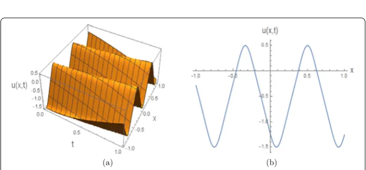
Figure 1(a) The 3D graph of a rational function solutionu(x,t) appearing in Eq. (29), whenκ= –6, ω=1₂t2₊_t_and_ξ

0= 1; (b) the corresponding 2D graph foru(x,t), whent= 1

Whenα1>α2orα1<α3,

Φ= 2h

(α2–α3)cosh[

√

h(ξ1–ξ0)] – (2α1–α2–α3)

, (81)

and then we have

φ(ξ) = 2a

–1₄ 4 h

(α2–α3)cosh[

√

h(a

1 4

4ξ–ξ0)] – (2α1–α2–α3) –b1

2. (82)

For instance, ifa4= 1,κ= –6,b1= 1,b(t) =t+ 1,p= –9,q= –4,r= 12, thenω(t) =1₂t2+

t+c. Settingc= 0, the solution can be obtained as

u(x,t) = 15

cosh[√15(–6x+1₂t2₊_t_–_ξ_{0)] + 4}– 1

2. (83)

3 Numerical simulations for modiﬁed Gardner equation

In this section, numerical simulations of modiﬁed Gardner equation are given. According to the solutions obtained above, each solution is chosen to carry out a typical numerical simulation, using Eqs. (29), (33), (37), (43), (53), (59), (67), (77) and (83). The 3D and the corresponding 2D graphs of are drawn to present the nature of them. In addition, we only focus on the positive one if there is a plus–minus sign in the selected solutions.

Case1. Fora4= 1, see Fig.1. Case2. Fora4= 1, see Fig.2. Case3. Fora4= 1, see Fig.3.

Case4. Fora4= 1, see Fig.4. Case5. Fora4= 1, see Fig.5. Case6. Fora4= 1, see Fig.6.

(12)

Figure 2(a) The 3D graph of a triangle function periodic solutionu(x,t) in Eq. (33), whenκ= –6,ω=1₂t2₊_t

andξ0= 1; (b) the corresponding 2D graph foru(x,t), whent= 1

Figure 3(a) The 3D graph of a rational function solutionu(x,t) illustrating Eq. (37), whenκ= –6,ω=1₂t2+t

Figure 4(a) The 3D graph of a hyperbolic cotangent function solutionu(x,t) demonstrating Eq. (43), when κ= –6,ω=1₂t2+tandξ0= 1; (b) the corresponding 2D graph foru(x,t), whent= 1

4 Conclusion

(13)

Figure 5(a) The 3D graph of Jacobi elliptic function solutionu(x,t) appearing in Eq. (53), whenκ= –6, ω=1

2t

2₊_t_and_ξ

Figure 6(a) The 3D graph of a solitary wave solutionu(x,t) reﬂected in Eq. (59), whenκ= –6,ω=1₂t2₊_t_and

ξ0= 1; (b) the corresponding 2D graph foru(x,t), when t = 1

Figure 7(a) The 3D graph of Jacobi elliptic function solutionu(x,t) illustrating Eq. (67), whenκ= –6, ω=1₂t2+tandξ0= 1; (b) the corresponding 2D graph foru(x,t), whent= 1

(14)

Figure 8(a) The 3D graph of Jacobi elliptic function solutionu(x,t) demonstrating Eq. (77), whenκ= –6, ω=1

2t

2₊_t_and_ξ

Figure 9(a) The 3D graph of a solitary wave solutionu(x,t) appearing in Eq. (83), whenκ= –6,ω=1₂t2₊_t

other methods. In addition, some solutions with the specific parameters are also presented in the paper, thus the existence of the solutions is proved. Our results may be helpful to better understand the two-layer fluid with surface tension, and the problem with specific boundary and initial conditions will be studied in a future work. Moreover, we can also conclude that the trial equation method and the discrimination system for polynomial method are powerful in solving differential equations with variable coefficients arising in mathematical physics.

Acknowledgements

The authors would like to thank the reviewers for their helpful comments and suggestions to improve the manuscript.

Funding

This work was ﬁnanced by Grant-in-aid for scientiﬁc research from the National Natural Science Foundation of China (NO. 51465047).

Competing interests

We would like to declare no conﬂicts of interest.

Authors’ contributions

(15)

Publisher’s Note

Springer Nature remains neutral with regard to jurisdictional claims in published maps and institutional aﬃliations.

Received: 6 December 2018 Accepted: 12 March 2019 References

1. Ablowitz, M.J., Clarkson, P.A.: Solitons, Nonlinear Evolutions and Inverse Scattering. Cambridge University Press, Cambridge (1991)

2. Liu, C.-S.: Canonical-like transformation method and exact solutions to a class of diﬀusion equations. Chaos Solitons Fractals42(1), 441–446 (2009)

3. Wadati, M.: Invariances and conservation laws of the Korteweg–de Vries equation. Stud. Appl. Math.59(2), 153–186 (1978)

4. Bulman, G.W., Sukeyuki, K.: Symmetries and Diﬀerential Equations. Springer, New York (1991)

5. Korteweg, D.J., de Vries, G.: On the change of form of long waves advancing in a rectangular canal, and on a new type of long stationary waves. Philos. Mag. Ser. 539, 422–443 (1895)

6. Ramollo, M.P.: Internal solitary waves in a two-layer ﬂuid with surface tension. Adv. Fluid Mech.9, 209–219 (1996) 7. Liu, Y., Gao, Y.-T., Sun, Z.-Y., Yu, X.: Multi-soliton solutions of the forced variable-coeﬃcient extended Korteweg–de

Vries equation arisen in ﬂuid dynamics of internal solitary waves. Nonlinear Dyn.66(4), 575–587 (2011) 8. Holloway, P.E., Pelinovsky, E., Talipova, T., Barnes, B.: A nonlinear model of internal tide transformation on the

Australian North West shelf. J. Phys. Oceanogr.27(6), 871–896 (1997)

9. Liu, C.-S.: Trial equation method and its applications to nonlinear evolution equations. Acta Phys. Sin.54(6), 2505–2509 (2005)

10. Liu, C.-S.: Using trial equation method to solve the exact solutions for two kinds of KdV equations with variable coeﬃcients. Acta Phys. Sin.54(10), 4506–4510 (2005)

11. Liu, C.-S.: Trial equation method to nonlinear evolution equations with rank inhomogeneous: mathematical discussions and its applications. Commun. Theor. Phys.45(2), 219–223 (2006)

12. Liu, C.-S.: A new trial equation method and its applications. Commun. Theor. Phys.45(3), 395–397 (2006) 13. Liu, C.-S.: Exponential function rational expansion method for nonlinear diﬀerential-diﬀerence equations. Chaos

Solitons Fractals40(2), 708–716 (2009)

14. Liu, C.-S.: Trial equation method based on symmetry and applications to nonlinear equations arising in mathematical physics. Found. Phys.41(5), 793–804 (2011)

15. Liu, C.-S.: Classiﬁcation of all single travelling wave solutions to Calogero–Degasperis–Focas equation. Commun. Theor. Phys.48(4), 601–604 (2007)

16. Liu, C.-S.: All single travelling wave solutions to Nizhnok–Novikov–Veselov equation. Commun. Theor. Phys.45(6), 991–992 (2006)

17. Liu, C.-S.: The classiﬁcation of travelling wave solutions and superposition of multi-solutions to Camassa–Holm equation with dispersion. Chin. Phys.16(7), 1832–1837 (2007)

18. Liu, C.-S.: Representations and classiﬁcations of travelling wave solutions to sinh-Gordon equation. Commun. Theor. Phys.49(1), 153–158 (2008)

19. Liu, C.-S.: Solution of ODEu+p(u)(u)2₊_q₍_u_{) = 0 and applications to classiﬁcations of all single travelling wave}

solutions to some nonlinear mathematical physics equations. Commun. Theor. Phys.49(2), 291–296 (2008) 20. Liu, C.-S.: Applications of complete discrimination system for polynomial for classiﬁcations of travelling wave

solutions to nonlinear diﬀerential equations. Comput. Phys. Commun.181(2), 317–324 (2010) 21. Bluman, G.W., Kumei, S.: Symmetries and Diﬀerential Equations. Springer, New York (1989) 22. Hirota, R.: The Direct Method in Soliton Theory. Cambridge University Press, Cambridge (2004)

23. Sierra, C.A.G., Molati, M., Ramollo, M.P.: Exact solutions of a generalized KdV–mKdV equation. Int. J. Nonlinear Sci. 13(1), 94–98 (2012)