R E S E A R C H
Open Access
Legendre spectral element method for
solving sine-Gordon equation
Mahmoud Lotfi
1*and Amjad Alipanah
1*Correspondence: lotfi[email protected] 1Department of Applied
Mathematics, University of Kurdistan, Sanandaj, Iran
Abstract
In this paper, we study the Legendre spectral element method for solving the sine-Gordon equation in one dimension. Firstly, we discretize the equation by Legendre spectral element in space and then discretize the time by the second-order leap-frog method. We study the stability and convergence of the method and show the convergence of our method. Finally, we show the results with numerical examples.
MSC: 65M70; 65M06; 74G15
Keywords: Sine-Gordon equation; Legendre spectral element method; Leap-frog method
1 Introduction
A spectral element method combines the high accuracy of spectral methods and flexi-bility of finite element method, and the approximate result of this method provides high accuracy and spectral convergence. In this method the solution is approximated on each element using spectral methods. One of the advantages of this method is the high accu-racy and stable solving algorithm with a small number of elements under a wide range of conditions [1].
Finite element method was proposed for the first time in 1943 by Courant [2]. He solved the Poisson equation based on minimizing piecewise linear approximations on finite sub-domains.
The spectral method is a conventional method for solving partial differential equations, which was first introduced by Navier for elastic sheet problems in 1825. In spectral method the solution is approximated on one general domain.
In 1984, Patera applied a spectral method to a greater number of subdomains by a divi-sion of domains. He proposed the spectral element method by combining the spectral method and the finite element method [3]. In his innovative method, Patera uses the Chebyshev polynomials as the interpolation basis functions. Legendre’s spectral element was developed by Maday and Patera [4]. The use of the Lagrangian interpolation conju-gate with the Gauss–Legendre–Lobatto quadrature leads to a matrix of mass with diam-eter structure [5]. The diagonal mass matrix is a very important property of the Legendre spectral element method and is different from the Chebyshev spectral element method [6]. The Legendre spectral element method is widely used in solving partial differential equations. Chen et al. [7] used the Legendre spectral element method to solve a
strained optimal control problem. An alternating direction implicit (ADI) Legendre spec-tral element method for the two-dimensional Schrodinger equation is developed in [8], and the optimal H1 error estimate for the linear case is given. The aim of [9] is the Lagrange–Galerkin spectral element method for solving two-dimensional shallow water equations. The authors of [10] considered the numerical approximation of the acoustic wave equation by the spectral element method based on the Gauss–Lobatto–Legendre quadrature formulas and finite difference Newmark’s explicit time advancing schemes. A modified set of basis functions for use with spectral element methods is presented in [11] for solving a mixed elliptic boundary value problem. These basis functions are constructed so that the axial conditions along a plane or axis of symmetry are satisfied identically. A numerical spectral element method for the computation of fluid flows governed by the incompressible Euler equations in a complex geometry is presented in [12]. Zhuang and Chen [13] used this method to solve biharmonic equations. In [14], the authors used the spectral element method with least-square formulation for parabolic interface problems. Ai et al. [15] used fully diagonalized Legendre spectral element methods using Sobolev orthogonal/biorthogonal basis functions for solving second-order elliptic boundary value problems. A Legendre spectral element formulation of an improved time-splitting method is developed for the natural convection heat transfer problem in a square cavity by Wang and Qin [16].
The sine-Gordon equation is one of the most important partial differential equations, which applies to many scientific fields such as the motion of a rigid pendula attached to a stretched wire [17], solid state physics, nonlinear optics, and the stability of fluid motions.
We consider the one-dimension sine-Gordon equation
utt–uxx+sin(u) = 0, x∈Ω,t∈(0,T),
ux(x,t) = 0, x∈∂Ω,t∈(0,T),
u(x, 0) =u0(x), ut(x, 0) =u1(x), x∈Ω,
(1)
whereuis a function ofxandt, andu0(x) andu1(x) are known analytic functions.
Different numerical methods are presented for Eq. (1). Dehghan and Shokri [18] solved a one-dimensional sine-Gordon equation using collocation points and approximating the solution using thin plate splines radial basis function. Dehghan and Mirzaei [19] used a numerical method of the boundary integral equation to approximate the solution of one-dimensional equation (1). Mohebbi and Dehghan [20] have also used the finite difference method for numerical solution of equation (1).
In [21] the authors present an analysis of the stability spectrum for all stationary periodic solutions to the sine-Gordon equation. Yousif an Mahmood [22] used the variational ho-motopy perturbation method for solving the Klein–Gordon and sine-Gordon equations. In [23] a new scheme, which has energy-preserving property, is proposed for solving the sine-Gordon equation with periodic boundary conditions. This method is obtained by the Fourier pseudo-spectral method and the fourth-order average vector field method. Baccouch [24] presented superconvergence results for the local discontinuous Galerkin method for the sine-Gordon nonlinear hyperbolic equation in one space dimension.
mul-tiquadric quasi-interpolation [27], reduced differential transform method [28], pseudo-spectral method [29], modified cubic B-spline differential quadrature method [30], mod-ified cubic B-spline collocation method [31], etc.
In this paper, we study the Legendre spectral element method for solving Eq. (1). First, using the Legendre spectral element method, we obtain a semi-discrete spatial form of Eq. (1), and then, using the leap-frog method, we obtain a complete discrete form of Eq. (1). We bring theorems on stability and convergence, and, finally, we show the results by a numerical example.
This paper is organized as follows: In Sect. 2, we perform a spatial discretization of Eq. (1) using the Legendre spectral element method. In Sect.3, we perform a time dis-cretization of Eq. (1) using the second-order leap-frog method. In Sect.4, we present sta-bility and convergence theorems. Finally, in Sect.5, we present a numerical example to validate the stability and convergence of the numerical scheme with respect to the dis-cretization parameters.
2 Space discretization
In this section, we explain the Legendre spectral element method and spatial discretization of Eq. (1).
2.1 Legendre spectral element method
In the Legendre spectral element method, we first divide the domainΩintoNe
nonover-lapping subdomainsΩe:
¯
We define the approximation space
Uh={u∈U:u|
Ωe∈PN},
wherePN is a polynomial space of dimension less than or equal toN. Basis functions are
considered as the Lagrangian interpolation polynomials defined at Gauss–Lobatto inte-gration points on each element. IfNe= 1, then we obtain the spectral Galerkin method of
orderN– 1. IfN= 1 orN= 2, then we obtain a standard Galerkin finite element method based on linear and quadratic elements, respectively.
Now on each elementΩe, we define the approximate solution of orderNas
ue(x,t) =
N
j=0
uej(t)ϕj(x), 1≤e≤Ne, (2)
where ϕj is thejth Lagrange polynomial of orderN on the Gauss–Legendre–Lobatto
points{ξi}Ni=0[32]:
To convert the [–1, 1] to theeth element and its inverse, we use the mapping functions
wherexeandxe–1are the endpoints of theeth element. The stiffness [33] and mass matrices
[34] on each element are calculated as follows:
Se
Using the Gauss quadrature, we obtain [35]
Seij= 2
2.2 Space discretization of the sine-Gordon equation
The second integral on the left-hand side is obtained by integration by parts. Now, taking thekth Lagrange function of orderNas the test functionvand using Eq. (2), we have
N
We obtain the right-hand side of Eq. (3) using the following equation [36]:
sinue∼=
The matrix form of the semidiscrete form of Eq. (3) is
MeUtte(t) +SeUe(t) = –MesinUe(t), (4) where the vectorUecontains an approximation solution of orderNon the elementΩ
e
at timet,Meis a local diagonal mass matrix, andSeis a local stiffness matrix on the
ele-mentΩe.
To obtain a semidiscrete form on the general domain, we must assemble the local ma-tricesMeandSeand obtain the general matricesMandS[35]. So Eq. (4) becomes
MUtt(t) +SU(t) = –Msin
U(t), (5)
whereUis the vector of the approximate solution on the general domainΩat timet.
3 Time discretization
For full discretization of Eq. (5), we first divide the interval (0,T) into subintervals [tn,tn+1],
wheret0= 0 andtn+1=tn+kforn= 0, . . . ,Nt– 1. Now, using the leap-frog method, we
obtain the full discrete form of Eq. (1):
MUn+1– 2Un+Un–1
k2 +SUn= –Msin(Un), (6)
where Unis the vector of approximation solution at time tn. After simplifying, Eq. (6)
For calculation ofU–1, we have
d dtU0=
U1–U–1
2k ,
and thus
U–1=U1– 2k
d dtU0.
So, forn= 0, we have
2MU1=
2M–k2SU0+ 2kM
d dtU0–k
2Msin(U
0). (8)
Forn> 0, we also have
MUn+1=
2M–k2SUn–MUn–1–k2Msin(Un). (9)
Because the mass matrixMis diagonal, solving Eqs. (8) and (9) is easier than by similar methods.
4 Stability and convergence analysis
In this section, we analyze the stability of leap-frog method and the convergence of the spectral element method presented in the previous sections.
4.1 Stability of leap-frog method Equation (9) can be written as
Un+1=
2I–k2AUn+Fn,n–1,
where
A=M–1S
and
Fn,n–1= –Un–1+k2sin(Un).
SinceFn,n–1is a known vector at each step and does not play any role in the stability
anal-ysis, we need to consider the equation
Un+1=
2I–k2AUn. (10)
Theorem 4.1 Equation(10)is stable under the following condition:
C∗N–1≤k2≤ ˜CN–3h2, h= max 1≤e≤Ne
Proof We must show that
2I–k2A22=ρ2I–k2A≤1.
Ifμiare the eigenvalues of the diagonal matrixMandλiare the eigenvalues of the matrix
S, then λi
μi are the eigenvalues of the matrixA. We must show that
2I–k2λi μi
≤1.
From this inequality we obtain
k–2≤ λi μi≤
3k–2. (11)
According to [37], we have that
C1N–1h≤λi≤C2N2h–1,
C3N–2h≤μi≤C4N–1h–2,
and, consequently,
C5N≤
λi
μi
≤C6N3h–2.
According to Eq. (11),
C∗N–1≤k2≤ ˜CN–3h2.
4.2 Convergence of spectral element method
In [38] the convergence theorem is presented for the spectral element method for acoustic waves.
Theorem 4.2([38]) Suppose that u∈C2(0,T;Hs(Ω))∩C4(0,T;L2(Ω))is the exact
solu-tion of
Mun+1– 2un+un–1
k2 +Sun= 0
and U is the approximation result of the spectral element method under stability conditions on k.Then,for all tn> 0,we have
u(tn) –UnL2(Ω)≤O
hmin(N,s)N–s+k2.
5 Numerical results
We set
whereNe,N are all nodes of the domain, andUnis the vector of nodal values of the
numer-ical solution corresponding to the discretization parametersN,Ne, andkat timetn, and
for each continuous functionf,
f2=
Example5.1 We consider the equation
utt–uxx+sin(u) = 0, –20≤x≤20,t≥0,
and the exact solution is given by
u(x,t) = 4arctan
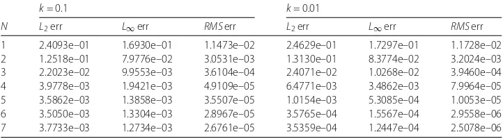
We solve this problem with the Legendre spectral element method presented in this paper with several values ofN,k, andNeat final timeT= 1. Table1shows the errors of Legendre
spectral element method with several values ofNat final timeT= 1 withk= 0.1, 0.01 and Ne= 20.
Table 2 shows the maximum pointwise error |uexact–uLSEM| at several times T =
1, 2, . . . , 10 withN= 4,Ne= 20, andk= 0.01.
Table 1 Numerical results for sine-Gordon equation Example5.1withNe= 20 andT= 1
k= 0.1 k= 0.01
N L2err L∞err RMSerr L2err L∞err RMSerr
1 2.4093e–01 1.6930e–01 1.1473e–02 2.4629e–01 1.7297e–01 1.1728e–02
2 1.2518e–01 7.9776e–02 3.0531e–03 1.3130e–01 8.3774e–02 3.2024e–03
3 2.2023e–02 9.9553e–03 3.6104e–04 2.4071e–02 1.0268e–02 3.9460e–04
4 3.9778e–03 1.9421e–03 4.9109e–05 6.4771e–03 3.4862e–03 7.9964e–05
5 3.5862e–03 1.3858e–03 3.5507e–05 1.0154e–03 5.3085e–04 1.0053e–05
6 3.5050e–03 1.3304e–03 2.8967e–05 3.5765e–04 1.5567e–04 2.9558e–06
Table 2 Maximum pointwise error at several times for sine-Gordon equation in Example5.1with N= 4,Ne= 20, andk= 0.01
Time (second) Max|uexact–uLSEM|
1 3.4862e–03
2 3.7742e–03
3 5.0095e–03
4 5.7173e–03
5 5.7173e–03
6 5.7173e–03
7 1.1208e–02
8 1.5732e–02
9 2.3081e–02
10 3.3925e–02
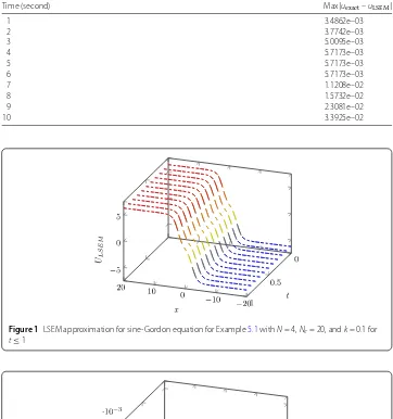
Figure 1LSEM approximation for sine-Gordon equation for Example5.1withN= 4,Ne= 20, andk= 0.1 for
t≤1
Figure 2Absolute error for sine-Gordon equation for Example5.1withN= 4,Ne= 20, andk= 0.1
Figures1and2show graphs of approximate solution and absolute error and Fig.3shows graph of approximate and exact solution atT= 1, using present method withN= 4,Ne=
20 andk= 0.1.
Figure 3Comparison between the LSEM and exact solutions for Example5.1atT= 1 withN= 4,Ne= 20 and
k= 0.1
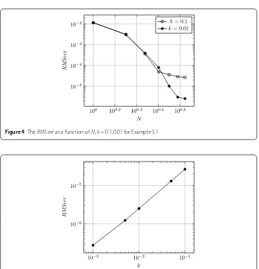
Figure 4TheRMSerr as a function ofN,k= 0.1, 0.01 for Example5.1
Figure 5TheRMSerr as a function ofk:N= 7,Ne= 20 for Example5.1
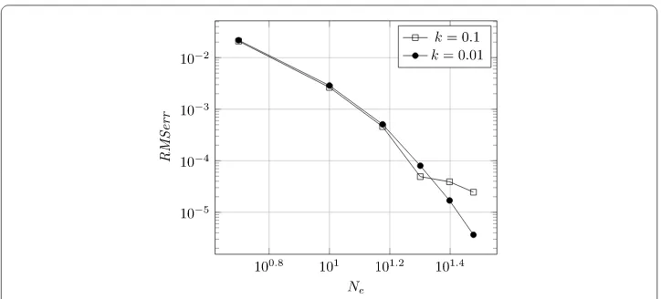
Figure 6TheRMSerr as a function ofNe:N= 4,k= 0.1, 0.01 for Example5.1
Table 3 Comparison ofL2err andL∞err of Example5.2withN= 7,Ne= 30, andk= 0.001 at different time levels
Time (s) LSEM Dehghan and Shokri [18] Shukla and Tamsir [30] Mittal and Bhatia [31]
L2err L∞err L2err L∞err L2err L∞err L2err L∞err
0.25 2.39e–06 4.05e–06 3.91e–05 5.89e–06 2.43e–06 5.56e–06 1.18e–05 2.32e–05
0.5 6.85e–06 7.02e–06 1.30e–04 2.01e–05 5.54e–06 7.39e–06 4.19e–05 4.11e–05
0.75 6.97e–06 7.36e–06 2.35e–04 3.63e–05 6.45e–06 7.40e–06 7.78e–05 1.02e–04
1 1.07e–05 2.23e–05 3.27e–04 5.07e–05 7.84e–06 8.75e–06 1.30e–04 1.64e–04
Figure6shows theRMSerras a function ofNefor two fixed values ofk(k= 0.1, 0.01)
andN= 4.
Example5.2 In this example, we obtain the numerical solutions of Eq. (1) the computa-tional domainΩ= [–1, 1] with the initial conditions
u(x, 0) = 0,
ut(x, 0) = 4sech(x).
(14)
The analytical solution is given in [39] as
u(x,t) = 4arctant·sech(x). (15)
The boundary conditions are obtained from the exact solution. We compute the numerical solution in the domainΩ= [–1, 1] with several values ofN,k,Ne, and timet. The obtained
results are compared with the results in [18,30,31]. Table3shows the results at the differ-ent time levels. It can be seen from Table3that the present results are in good agreement with those in the literature. A graph comparing the exact and numerical solutions atT= 1 withN= 4,k= 0.01, andNe= 20 is depicted in Fig.7. We also draw the space-time graph
Figure 7Comparison between the LSEM and exact solutions for Example5.2att= 1 withN= 4,Ne= 20, and
k= 0.01
Figure 8LSEM approximation for sine–Gordon equation Example5.2withN= 2,Ne= 10, andk= 0.01 for
t≤2
Example5.3 Consider the sine-Gordon equation (1) in the rangeΩ= [–10, 10] with the initial conditions
⎧ ⎨ ⎩
u(x, 0) = 0,
ut(x, 0) = 4γsech(γx),
(16)
wherec= 0.5 is the velocity of solitary wave, andγ =√1
1+c2. The exact solution [31] is given
as
u(x,t) = 4arctanc–1sin(γct)sech(γx). (17)
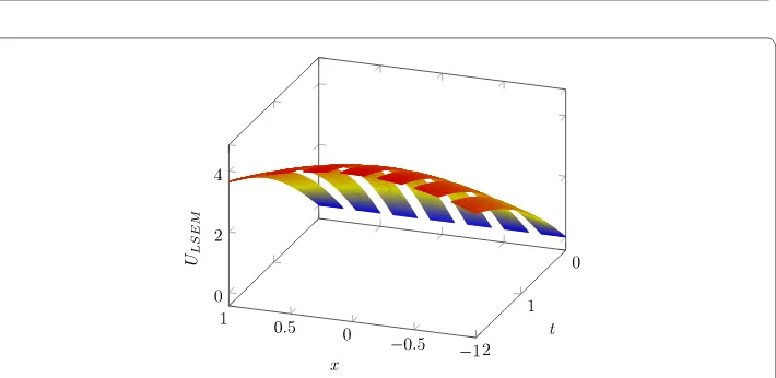
The boundary conditions can be obtained from the exact solution. The numerical solution for Example5.3is computed in the domain [–10, 10] using the parameter valuesN= 7, Ne= 30, andk= 0.001. Computed results are compared with the results obtained in [30,
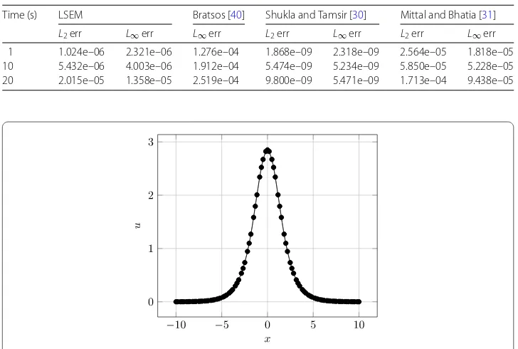
31,40]. Table4showsL2errandL∞errat different time levels. From Table4we can see that
Table 4 Comparison of theL2err andL∞err of Example5.3withN= 7,Ne= 30, andk= 0.001 at
different time levels
Time (s) LSEM Bratsos [40] Shukla and Tamsir [30] Mittal and Bhatia [31]
L2err L∞err L∞err L2err L∞err L2err L∞err
1 1.024e–06 2.321e–06 1.276e–04 1.868e–09 2.318e–09 2.564e–05 1.818e–05
10 5.432e–06 4.003e–06 1.912e–04 5.474e–09 5.234e–09 5.850e–05 5.228e–05
20 2.015e–05 1.358e–05 2.519e–04 9.800e–09 5.471e–09 1.713e–04 9.438e–05
Figure 9Comparison between the LSEM and exact solutions for Example5.3att= 1 withN= 3,Ne= 30 and
k= 0.01
Figure 10 LSEM approximation for sine-Gordon equation Example5.3withN= 3,Ne= 30 andk= 0.1, for
t≤10
withN= 3,Ne= 30, andk= 0.01. In Fig.10, we show the space-time graph of approximate
solution fort≤10 using the present method withN= 3,Ne= 30, andk= 0.1.
6 Conclusion and discussion
sine-Gordon equation. We used the Legendre spectral element method for discretizing the spatial space. Also, we used a leap-frog scheme for discretizing the temporal space with the stability conditionC∗N–1≤k2≤ ˜CN–3h2. We presented theorems on the
stabil-ity and convergence. Finally, using one test problem, we demonstrated that the algorithm is efficient for obtaining approximation solutions of the sine-Gordon equation.
Acknowledgements
The authors are thankful to the honorable reviewers and editors for their valuable suggestions and comments, which improved the paper.
Funding Not applicable.
Availability of data and materials
The results and numerical data obtained in this paper have been fully tested. These results are obtained using MATLAB R2017a(win64) software and Windows 8 operating system on a intel(R) Core(TM) i7 CPU, 1.73 GHz processor with 4 GB RAM. The authors declare that all data and material in the paper are available and veritable.
Competing interests
The authors declare that they have no competing interests.
Authors’ contributions
Both authors contributed equally and significantly in writing this article. Both authors wrote, read, and approved the final manuscript.
Publisher’s Note
Springer Nature remains neutral with regard to jurisdictional claims in published maps and institutional affiliations.
Received: 27 September 2018 Accepted: 7 March 2019
References
1. Vosse, F.N., Minev, P.D.: Spectral Element Methods: Theory and Applications. Eindhoven University of Technology, EUT Report 96-w-001 (1996)
2. Courant, R.: Variational method for the solution of problems of equilibrium and vibration. Bull. Am. Math. Soc.49, 1–23 (1943)
3. Patera, A.T.: A spectral element method for fluid dynamics: laminar flow in a channel expansion. J. Comput. Phys.54, 468–488 (1984)
4. Maday, Y., Patera, A.T.: Spectral Element Methods for the Incompressible Navier–Stokes Equations, Surveys on Computational Mechanics. ASME, New York (1989)
5. Bathe, K.J.: Finite Element Procedures, 2nd edn. Prentice Hall International, Englewood Cliffs (1995) 6. Priolo, E., Seriani, G.A.: A numerical investigation of Chebyshev spectral element method for acoustic wave
propagation. In: Proceedings of the 13th IMACS Conference Comparat, vol. 54, pp. 154–172 (1991)
7. Chen, Y., Yi, N., Liu, W.: A Legendre–Galerkin spectral method for optimal control problems governed by elliptic equations. SIAM J. Numer. Anal.46, 2254–2275 (2008)
8. Zeng, F., Ma, H., Zhao, T.: Alternating direction implicit Legendre spectral element method for Schrödinger equations. J. Shanghai Univ. Nat. Sci. Ed.17(6), 724–727 (2011)
9. Giraldo, F.X.: Strong and weak Lagrange–Galerkin spectral element methods for the shallow water equations. Comput. Math. Appl.45, 97–121 (2003)
10. Zampieri, E., Pavarino, L.F.: Approximation of acoustic waves by explicit Newmark’s schemes and spectral element methods. J. Comput. Appl. Math.185, 308–325 (2006)
11. VanOs, R.G., Phillips, T.N.: The choice of spectral element basis functions in domains with an axis of symmetry. J. Comput. Appl. Math.201, 217–229 (2007)
12. Xu, C., Maday, Y.: A spectral element method for the time-dependent two-dimensional Euler equations: applications to flow simulations. J. Comput. Appl. Math.91, 63–85 (1998)
13. Zhuang, Q., Chen, L.: Legendre–Galerkin spectral-element method for the biharmonic equations and its applications (in press)
14. Khan, A., Upadhyay, C.S., Gerritsma, M.: Spectral element method for parabolic interface problems. Comput. Methods Appl. Mech. Eng. (2018).https://doi.org/10.1016/j.cma.2018.03.011
15. Ai, Q., Li, H.Y., Wang, Z.Q.: Diagonalized Legendre spectral methods using Sobolev orthogonal polynomials for elliptic boundary value problems. Appl. Numer. Math. (2018).https://doi.org/10.1016/j.apnum.2018.01.003
16. Wang, Y., Qin, G., Wang, Z.Q.: An improved time-splitting method for simulating natural convection heat transfer in a square cavity by Legendre spectral element approximation. Comput. Fluids (2018).
https://doi.org/10.1016/j.compfluid.2018.07.013
17. Wazwaz, A.M.: A variable separated ODE method for solving the triple sine-Gordon and the triple sinh-Gordon equations. Chaos Solitons Fractals33, 703–710 (2007)
19. Dehghan, M., Mirzaei, D.: The boundary integral equation approach for numerical solution of the one-dimensional sine-Gordon equation. Numer. Methods Partial Differ. Equ.24, 1405–1415 (2008)
20. Mohebbi, A., Dehghan, M.: High order solution of one-dimensional sine-Gordon equation using compact finite difference and DIRKN methods. Math. Comput. Model.51, 537–549 (2010)
21. Deconinck, B., McGil, P., Sega, B.L.: The stability spectrum for elliptic solutions to the sine-Gordon equation. Physica D
360, 17–35 (2017)
22. Yousif, M.A., Mahmood, B.A.: Approximate solutions for solving the Klein–Gordon and sine-Gordon equations. J. Assoc. Arab Univ. Basic Appl. Sci.22, 83–90 (2017)
23. Jiang, C., Sun, J., Li, H., Wang, Y.: A fourth-order AVF method for the numerical integration of sine-Gordon equation. Appl. Math. Comput.313, 144–158 (2017)
24. Baccouch, M.: Superconvergence of the local discontinuous Galerkin method for the sine-Gordon equation in one space dimension. J. Comput. Appl. Math.333, 292–313 (2018)
25. Shao, W., Wu, X.: The numerical solution of the nonlinear Klein–Gordon and sine-Gordon equations using the Chebyshev tau meshless method. Comput. Phys. Commun.185, 1399–1409 (2014)
26. Hussain, A., Haq, S., Uddin, M.: Numerical solution of Klein–Gordon and sine-Gordon equations by meshless method of lines. Eng. Anal. Bound. Elem.37, 1355–1366 (2013)
27. Jiang, Z.W., Wang, R.H.: Numerical solution of one-dimensional sine-Gordon equation using high accuracy multiquadric quasi-interpolation. Appl. Math. Comput.218, 7711–7716 (2012)
28. Keskin, Y., Aglar, I., Ko, A.: Numerical solution of sine-Gordon equation by reduced differential transform method, vol. 1 (2011)
29. Taleei, A., Dehghan, M.: A pseudo-spectral method that uses an overlapping multidomain technique for the numerical solution of sine-Gordon equation in one and two spatial dimensions. Math. Methods Appl. Sci.37, 1909–1923 (2014)
30. Shukla, H.S., Tamsir, M.: Numerical solution of nonlinear sine-Gordon equation by using the modified cubic B-spline differential quadrature method. Beni-Suef Univ. J. Basic Appl. Sci.7(4), 359–366 (2018)
31. Mittal, R.C., Bhatia, R.: Numerical solution of nonlinear sine-Gordon equation by modified cubic B-spline collocation method. Int. J. Partial Differ. Equ. (2014).https://doi.org/10.1155/2014/343497
32. Hesthaven, J.S., Gottlieb, S., Gottlieb, D.: Spectral Method for Time-Dependent Problems. Cambridge University Press, Cambridge (2007)
33. Ern, A., Guermond, J.L.: Theory and Practice of Finite Elements. Springer, New York (2004) 34. Hand, L.N., Finch, J.D.: Analytical Mechanics. Cambridge University Press, Cambridge (2008)
35. Pozrikidis, C.: Introduction to Finite and Spectral Element Methods Using Matlab. Chapman & Hall, London (2005) 36. Argyris, J., Haase, M., Heinrich, J.C.: Finite element approximation to two dimensional sine-Gordon solitons. Comput.
Methods Appl. Mech. Eng.86, 1–26 (1991)
37. Bernardi, C., Maday, Y.: Approximations Spectrales de Problèmes aux Limites Elliptiques. Springer, Berlin (1992) 38. Zampieri, E., Pavarino, L.F.: An explicit second order spectral element method for acoustic waves. Adv. Comput. Math.
25, 381–401 (2006)
39. Wei, G.W.: Discrete singular convolution for the sine-Gordon equation. Physica D137, 247–259 (2000)
40. Bratsos, A.G.: A fourth order numerical scheme for the one dimensional sine-Gordon equation. Int. J. Comput. Math.