Inequalities among Eigenvalues of Second Order Difference Equations with General Coupled Boundary Conditions

(1)

doi:10.1155/2009/347291

Research Article

Inequalities among Eigenvalues of

Second-Order Difference Equations with

General Coupled Boundary Conditions

Chao Zhang and Shurong Sun

School of Science, University of Jinan, Jinan, Shandong 250022, China

Correspondence should be addressed to Chao Zhang,ss [email protected]

Received 11 February 2009; Accepted 11 May 2009

Recommended by Johnny Henderson

This paper studies general coupled boundary value problems for second-order difference equations. Existence of eigenvalues is proved, numbers of their eigenvalues are calculated, and their relationships between the eigenvalues of second-order difference equation with three different coupled boundary conditions are established.

Copyrightq2009 C. Zhang and S. Sun. This is an open access article distributed under the Creative Commons Attribution License, which permits unrestricted use, distribution, and reproduction in any medium, provided the original work is properly cited.

1. Introduction

Consider the second-order diﬀerence equation

−∇pnΔyn

qnynλwnyn, n∈0, N−1 1.1

with the general coupled boundary condition

yN−1

ΔyN−1

eiαK

y₋₁ Δy−1

, 1.2

whereN ≥ 2 is an integer,Δis the forward diﬀerence operator:Δyn yn1−yn,∇is the backward diﬀerence operator: ∇yn yn −yn−1, andpn, qn,and wn are real numbers with

(2)

parameter; the interval 0, N −1 is the integral set{n}N_n−1₀; α, −π < α ≤ π is a constant parameter;i√−1,

K

k11 k12

k21 k22

, kij ∈R, i, j1,2, with detK1. 1.3

The boundary condition 1.2 contains the periodic and antiperiodic boundary conditions. In fact, 1.2 is the periodic boundary condition in the case where α 0 and

KI, the identity matrix, and1.2 is the antiperiodic condition in the case whereαπand

KI.

We first briefly recall some relative existing results of eigenvalue problems for diﬀerence equations. Atkinson1, Chapter 6, Section 2discussed the boundary conditions

y−1αym−1, ymβy0 1.4

when he investigated the recurrence formula

cnyn1

anλbn

yn−cn−1yn−1, n∈0, m−1, 1.5

wherean,bn,cn,α,andβare real numbers, subject toan>0, cn>0,and

αc−1βcm−1. 1.6

He remarked that all the eigenvalues of the boundary value problem1.4 and1.5 are real, and they may not be all distinct. If c−1 cm−1 and α β 1, he viewed the boundary conditions1.4 as the periodic boundary conditions for1.5. Shi and Chen2investigated the more general boundary value problem

−∇CnΔxn Bnxnλwnxn, n∈1, N, N≥2, 1.7

R

−x0

xN

S

C0Δx0

CNΔxN

0, 1.8

where Cn, Bn, and wn are d×dHermitian matrices; C0 and CN are nonsingular; wn > 0 for n ∈ 1, N;R and S are 2d×2d matrices. Moreover,R and S satisfy rankR, S 2d

(3)

see4, Theorems 2.2 and 3.1 : the periodic and antiperiodic boundary value problems have exactlyNreal eigenvalues{λi}Ni0−1and{λi}Ni1, respectively, which satisfy

λ0<λ1≤λ2 < λ1≤λ2<λ3≤λ4<· · ·< λN−2≤λN−1<λN, ifN is odd,

λ0<λ1≤λ2< λ1≤λ2 <λ3≤λ4<· · ·<λN−1≤λN< λN−1, ifN is even.

1.9

These results are similar to those about eigenvalues of periodic and antiperiodic boundary value problems for second-order ordinary diﬀerential equationscf.5–8 .

Motivated by4, we compare the eigenvalues of the eigenvalue problem1.1 with the coupled boundary condition 1.2 as α varies and obtain relationships between the eigenvalues in the present paper. These results extend the above results obtained in4. In this paper, we will apply some results obtained by Shi and Chen2to prove the existence of eigenvalues of1.1 and1.2 to calculate the number of these eigenvalues, and to apply some oscillation results obtained by Agarwal et al.9to compare the eigenvalues asαvaries. This paper is organized as follows. Section 2 gives some preliminaries including existence and numbers of eigenvalues of the coupled boundary value problems, and some properties of eigenvalues of a kind of separated boundary value problem, which will be used in the next section. Section 3 pays attention to comparison between the eigenvalues of problem1.1 and1.2 asαvaries.

2. Preliminaries

Equation1.1 can be rewritten as the recurrence formula

pnyn1

pnpn−1qn−λwn

yn−pn−1yn−1, n∈0, N−1. 2.1

Clearly,ynis a polynomial inλwith real coeﬃcients sincepn, qn,andwnare all real. Hence, all the solutions of1.1 are entire functions ofλ. Especially, ify0/0,yn is a polynomial of degreeninλforn≤N. However, ify−1/0 andy00,ynis a polynomial of degreen−1 in

λforn≤N.

We now prepare some results that are useful in the next section. The following lemma is mentioned in4, Theorem 2.1.

Lemma 2.14, Theorem 2.1 . Letyandzbe any solutions of1.1 . Then the Wronskian

Wy, zn yn1 zn1 pnΔyn pnΔzn

−pn

yn1zn−ynzn1

2.2

is a constant on−1, N−1.

Theorem 2.2. Ifk11/k12 then the coupled boundary value problem1.1 and1.2 has exactlyN

(4)

Proof. By settingd1,Cnpn,Bnqn,

R R1, R2

eiα_k

11 1

eiα_k

21 0

, S S1, S2

−eiα_k

12 0

−eiα_k

22 1

, 2.3

shifting the whole interval1, Nleft by one unit, and usingp−1 pN−1 1,1.1 and1.2 are written as1.7 and1.8, respectively. It is evident that rankR, S 2dandRS∗ SR∗. Hence, the boundary condition1.2 is self-adjoint by2, Lemma 2.1. In addition, it follows from2.3 andC₋₁1 that

R1S1C−1, S2

eiα_k

11−k12 0

eiαk21−k22 1

. 2.4

By noting thatk11/k12, we get rankR1S1C−1, S2 2. Therefore, by2, Theorem 4.1, the

problem1.1 and1.2 has exactlyNreal eigenvalues. This completes the proof.

Letynλ be the solution of1.1 with the initial conditions

y₋₁λ 0, y0λ /0. 2.5

Consider the sequence

y0λ , y1λ , . . . , yN−1λ . 2.6

Ifynλ 0 for somen ∈ 0, N−1 , then, we get from 2.1 thatyn−1λ andyn1λ have

opposite signs. Hence, we say that sequence2.6 exhibits a change of sign ifynλ yn1λ <0

for somen∈0, N−1 , orynλ 0 for somen∈0, N−1 . A general zero of the sequence

2.6 is defined as its zero or a change of sign.

Now we consider1.1 with the following separated boundary conditions:

y₋₁0, k12ΔyN−1−k22yN−10, 2.7

where k12, k22 are entries of K. It follows from 2.1 that the separated boundary value

problem1.1 with2.7 has a unique solution, and the separated boundary value problem will be used to compare the eigenvalues of1.1 and1.2 asαvaries in the next section.

In9, Agarwal et al. studied the following boundary value problem on time scales:

yΔΔqt yσ −λyσ, t∈ρa , ρb ∩T, 2.8

with the boundary conditions

Ra

y:αyρa βyΔρa 0, Rb

(5)

whereTis a time scale, σt and ρt are the forward and backward jump operators in T,

yΔ is the delta derivative, andyσ_t _: _yσt_; _q _: _{ρa , ρb}_∩_T _→ _R _{is continuous;}

α2_β2_γ2_δ2 _/_0;_{a, b}_∈_T_with_{a < b}_{. They obtained some useful oscillation results. With}

a similar argument to that used in the proof of9, Theorem 1, one can show the following result.

Lemma 2.3. The eigenvalues of the boundary value problem are

−pt yΔ_tΔ_qσ_{t y}σ_t_λrσ_{t y}σ_{t ,} _t_∈_{ρa , ρb}_∩_T, _2.10

with

Ra

yRb

y0, 2.11

wherepΔ, qσ_,_and_rσ _{are real and continuous functions in}_{ρa , ρb}_∩_{T, p >}₀_over_{ρa , b}_∩

T, rσ _>₀_over_{ρa , ρb}_∩_{T, pρa}_pb₁_{are arranged as}_−∞_{< λ}

0< λ1 < λ2 <· · · ,and

an eigenfunction corresponding toλkhas exactlykgeneralized zeros in the open intervala, b .

By settingρa , b∩T −1, N−1: {n}₋₁N−1,α 1, β 0, γ −k22, δ k12, the

above boundary value problem can be written as1.1 with2.7, then we have the following result.

Lemma 2.4. The boundary value problem1.1 and2.7 hasN−1 real and simple eigenvalues as

k12 0andNreal and simple eigenvalues ask12/0, which can be arranged in the increasing order

μ0< μ1<· · ·< μNs, whereNs:N−2 orN−1. 2.12

Letynλ be the solution of 1.1 with the separated boundary conditions2.7 . Then sequence2.6

exhibits no changes of sign forλ≤μ0, exactlyk1changes of sign forμk< λ≤μk1 0≤k≤Ns−1 ,

andNs1changes of sign forλ > μNs.

Letϕnandψnbe the solutions of1.1 satisfying the following initial conditions:

ϕ−1 ψ01, ϕ0ψ−10, 2.13

respectively. ByLemma 2.1and usingpN−11, we have

ΔϕN−1ψN−1−ϕN−1ΔψN−1ϕNψN−1−ϕN−1ψN−1. 2.14

(6)

Lemma 2.5. Letμk 0≤k≤Ns be the eigenvalues of1.1 and2.7 withk120and be arranged

as2.12 . Then,ψnμk is an eigenfunction of the problem1.1 and2.7 with respect toμk 0≤k≤

Ns , that is, for0≤k≤Ns,ψnμk is a nontrivial solution of 1.1 satisfying

ψ−1μk

ψN−1μk

0. 2.15

Moreover, ifkis odd,ψNμk >0and ifkis even,ψNμk <0for2≤k≤Ns.

A representation of solutions for a nonhomogeneous linear equation with initial conditions is given by the following lemma.

Lemma 2.6see4, Theorem 2.3 . For any{fn}nN−10 ⊂Cand for anyc−1, c0∈C, the initial value

problem

−∇pnΔzn

qn−λwn

znwnfn, n∈0, N−1,

z−1c−1, z0c0

2.16

has a unique solutionz, which can be expressed as

znc−1ϕnc0ψn n−1

j0

wj

ϕnψj−ϕjψn

fj, n∈−1, N, 2.17

where−2_j₀·−1_j₀·:0.

3. Main Results

Letϕnandψnbe defined inSection 2, letμk0≤k≤Ns be the eigenvalues of the separated boundary value problem1.1 with2.7 , and letλjeiαK 0≤j ≤N−1 be the eigenvalues of the coupled boundary value problem1.1 and1.2 and arranged in the nondecreasing order

λ0

eiαK≤λ1

eiαK≤ · · · ≤λN−1

eiαK. 3.1

Clearly,λjK 0 ≤ j ≤ N−1 denotes the eigenvalue of the problem1.1 and1.2 with

α0, andλj−K 0≤j≤N−1 denotes the eigenvalue of the problem1.1 and1.2 with

(7)

Theorem 3.1. Assume that k11 > 0, k12 ≤ 0 or k11 ≥ 0, k12 < 0. Then, for every fixedα /0,

−π < α < π, one has the following inequalities:

λ0K < λ0

eiα_K_{< λ}

0−K ≤λ1−K < λ1

eiα_K_{< λ}

1K

≤λ2K < λ2

eiαK< λ2−K

≤λ3−K < λ3

eiαK< λ3K

≤ · · · ≤λN−2−K < λN−2

eiαK< λN−2K

≤λN−1K < λN−1

eiαK< λN−1−K , ifN is odd,

λ0K < λ0

eiαK< λ0−K ≤λ1−K < λ1

eiαK< λ1K

≤λ2K < λ2

eiαK< λ2−K

≤λ3−K < λ3

eiαK< λ3K

≤ · · · ≤λN−2K < λN−2

eiαK< λN−2−K

≤λN−1−K < λN−1

eiα_K_{< λ}

N−1K , ifN is even.

3.2

Remark 3.2. Ifk11≤0, k12>0 ork11 <0, k12≥0, a similar result can be obtained by applying

Theorem 3.1to−K. In fact,eiα_K_eiπα₋_K_for_α_∈₋_π,₀ _and_eiα_K_ei−πα₋_K_for_α_∈

0, π . Hence, the boundary condition1.2 in the cases ofk11 ≤0, k12 >0 ork11 <0, k12 ≥0

andα /0,−π < α < π, can be written as condition1.2 , whereαis replaced byπαfor

α∈−π,0 and−παforα∈0, π , andKis replaced by−K.

Before provingTheorem 3.1, we prove the following five propositions.

Proposition 3.3. Forλ∈C,λis an eigenvalue of1.1 and1.2 if and only if

fλ 2 cosα, 3.3

where

fλ :k22ϕN−1λ k11−k12 ΔψN−1λ −k21−k22 ψN−1λ −k12ΔϕN−1λ . 3.4

Moreover,λis a multiple eigenvalue of 1.1 and1.2 if and only if

ϕN−1λ eiαk11−k12 , ΔϕN−1λ eiαk21−k22 ,

ψN−1λ eiαk12, ΔψN−1λ eiαk22.

(8)

Proof. Sinceϕnandψnare linearly independent solutions of1.1 , thenλis an eigenvalue of the problem1.1 and1.2 if and only if there exist two constantsC1andC2not both zero

such thatC1ϕnC2ψnsatisfies1.2, which yields

ϕN−1λ −eiαk11−k12 ψN−1λ −eiαk12

ΔϕN−1λ −eiαk21−k22 ΔψN−1λ −eiαk22

C1

C2

0. 3.6

It is evident that3.6 has a nontrivial solutionC1, C2 if and only if

det

ϕN−1λ −eiαk11−k12 ψN−1λ −eiαk12

ΔϕN−1λ −eiαk21−k22 ΔψN−1λ −eiαk22

0 3.7

which, together with2.14 and detK1, implies that

1e2iα−eiαfλ 0. 3.8

Then3.3 follows from the above relation and the fact thate−iα_eiα _{2 cos}_α_{. On the other} hand,1.1 has two linearly independent solutions satisfying1.2 if and only if all the entries of the coeﬃcient matrix of3.6 are zero. Hence,λis a multiple eigenvalue of1.1 and1.2 if and only if3.5 holds. This completes the proof.

The following result is a direct consequence of the first result ofProposition 3.3.

Corollary 3.4. For anyα∈−π, π,

λj

eiαKλj

e−iαK, 0≤j≤N−1. 3.9

Proposition 3.5. Assume thatk11 > 0, k12 ≤ 0or k11 ≥ 0, k12 < 0. Then one has the following

results.

i For eachk,0≤k≤Ns,fμk ≥2ifkis odd, andfμk ≤ −2ifkis even.

ii There exists a constantν0< μ0such thatfν0 ≥2.

iii If the boundary value problem 1.1 and2.7 has exactlyN−1eigenvalues then there exists a constantξ0such thatμN−2 < ξ0andfξ0 ≤ −2, whereNis odd, and there exists

a constantη0such thatμN−2< η0andfη0 ≥2, whereNis even.

Proof. i If ψnμk is an eigenfunction of the problem 1.1 and 2.7 respect to μk then

k12ΔψN−1μk −k22ψN−1μk 0. By Lemma 2.3and the initial conditions2.13 , we have that ifk12<0 then the sequenceψ0μk ,ψ1μk , . . . , ψN−1μk exhibitskchanges of sign and

sgnψN−1μk

(9)

(10)

Case 2. Ifk120 then it follows from2.7 and2.14 that for eachk, 0≤k≤Ns,

ϕN−1μk

ψN

μk

1. 3.17

From2.15 and by the definition offλ , we get

fμk

k22

ψN

μk

k11ψN

μk

. 3.18

Hence, noting detKk11k22 1,k11>0, and byLemma 2.5, we have that ifkis odd, then

fμk

≥2, 3.19

and ifkis even, then

fμk

≤ −2. 3.20

ii By the discussions in the first paragraph ofSection 2,ϕN−1λ is a polynomial of

degreeN−2 inλ,ϕNλ is a polynomial of degreeN−1 inλ,ψN−1λ is a polynomial of degreeN−1 inλ, andψNλ is a polynomial of degreeNinλ. Further,ψNλ can be written as

ψNλ −1 NANλNAN−1λN−1· · ·A0, 3.21

whereANw0w1· · ·wN−1p0p1· · ·pN−1 −1>0 andAnis a certain constant forn∈0, N−1. Then

fλ −1 Nk11−k12 ANλNhλ , 3.22

wherehλ is a polynomial inλwhose degree is not larger thanN−1. Clearly, asλ → −∞,

fλ → ∞sincek11 −k12 > 0. By the first part of this proposition,fμ0 ≤ −2. So there

exists a constantν0< μ0such thatfν0 ≥2.

iii It follows from the first part of this proposition that ifNis odd,fμN−2 ≥2 and

ifN is even,fμN−2 ≤ −2. By3.22 , if Nis odd,fλ → −∞asλ → ∞; ifN is even,

fλ → ∞asλ → ∞. Hence, if N is odd, there exists a constantξ0 > μN−2 such that

fξ0 ≤ −2; ifNis even, there exists a constantη0 > μN−2such thatfη0 ≥2. This completes

the proof.

Sinceϕnandψnare both polynomials inλ, so isfλ . Denote

d

dλfλ :f

_{λ ,} d2

(11)

Proposition 3.6. Assume thatk11 > 0, k12 ≤ 0 or k11 ≥ 0, k12 < 0. Equationsfλ 0 and

Diﬀerentiating3.25 and3.26 with respect toλ, respectively, yields that

−∇pnΔϕnλ

It follows from2.13 that

ϕ₀ϕ₋₁ψ₀ ψ₋₁ 0. 3.28

It follows from3.29 that

(12)

Hence, not indicatingλexplicitly, we get

(13)

linearly independent,δjλ is identically zero if and only if all the entries of the matrixIλ vanish, namely,

k12ΔψN−1λ −k22ψN−1λ 0,

k11−k12 ΔϕN−1λ −k21−k22 ϕN−1λ 0,

k22ϕN−1λ −k11−k12 ΔψN−1λ k21−k22 ψN−1λ −k12ΔϕN−1λ 0

3.34

which, together withfλ 2 and det K1, implies

ϕN−1λ k11−k12, ΔϕN−1λ k21−k22,

ψN−1λ k12, ΔψN−1λ k22.

3.35

Then byProposition 3.3,λis a multiple eigenvalue of1.1 and1.2 withα0. In addition,

3.34 , together withfλ −2 and detK1, implies

ϕN−1λ −k11−k12 , ΔϕN−1λ −k21−k22 ,

ψN−1λ −k12, ΔψN−1λ −k22.

3.36

Then byProposition 3.3,λis a multiple eigenvalue of1.1 and1.2 withαπ. Conversely, from3.35 or3.36 , it can be easily verified that3.34 holds, thenfλ 0. It follows again from3.35 or3.36 thatfλ 2 orfλ −2. Thusfλ 0 andfλ 2 or−2 if and only ifλis a multiple eigenvalue of1.1 and1.2 withα0 orαπ.

Further, for every fixedλwithfλ 2 or−2, not indicatingλexplicitly,3.33 implies that

k12ΔψN−1−k22ψN−1k11−k12 ΔϕN−1−k21−k22 ϕN−1

k22ϕN−1−k11−k12 ΔψN−1 k21−k22 ψN−1−k12ΔϕN−1

2

4 .

3.37

Therefore, from3.37 and by the definition ofδj, we have

δj

k12ΔψN−1−k22ψN−1

·

ϕj

2k12ΔψN−1−k22ψN−1 ψj

2 _3.38

and consequently, not indicatingλexplicitly, we have

fk12ΔψN−1−k22ψN−1

·N−1

j0

wj

ϕj

2k12ΔψN−1−k22ψN−1

ψj

2 _3.39

(14)

ν0_λ 0Kλ0e

iα_K

λ0−K μ0 λ1−K

−2 2 cosα 2

fλ

λ1eiαK μ1,λ1,2K λ2eiαK

λ2−K

λ

Figure 1:The graph offλ .

Suppose thatfλ 2 or−2 for someλ /μk 0 ≤ k ≤ Ns , we havek12ΔψN−1λ −

k22ψN−1λ /0.From the above discussions again,λis a simple eigenvalue of1.1 and1.2 withα0 orαπ, andδjis not identically zero for 0≤j≤N−1.

For thisλ /μk 0 ≤ k ≤ Ns ,3.39 implies that fλ /0, and from Proposition 3.5

i ,ii thatfμ0 ≤ −2,fν0 ≥ 2. Hence, fλ < 0, whereν0 < λ < μ0. It follows from

Proposition 3.5i thatfμk fμk1 ≤ −4 and−1 kfλ > 0, whereμk < λ < μk1 0≤ k ≤

N−3 . ByProposition 3.5i ,iii ,fμN−2 ≥2 and there existsμN−2< ξ0such thatfξ0 ≤ −2

ifN is odd, andfμN−2 ≤ −2 and there existsμN−2 < η0 such thatfη0 ≥ 2 ifNis even.

Hence,−1 N−2fλ >0 whereμN−2< λ. This completes the proof.

Proposition 3.7. For any fixedα /0,−π < α < π, each eigenvalue of1.1 and1.2 is simple.

Proof. Fixα,−π < α < πwithα /0. Suppose thatλis an eigenvalue of the problem1.1 and

1.2 . ByProposition 3.3, we havef2_λ_{4 cos}2_{α <}_{4. It follows from}_3.33 _{that det}_Iλ_>₀

and the matrixIλ is positive definite or negative definite. Hence,δj>0 for 0≤j≤N−1 or

δj<0 for 0≤j ≤N−1 sinceϕnandψnare linearly independent.

If λ is a multiple eigenvalue of problem 1.1 and 1.2, then 3.5 holds by Proposition 3.3. By using3.5 , it can be easily verified that3.34 holds, that is, all the entries of the matrixIλ are zero. Thenδj 0 for 0 ≤ j ≤ N−1, which is contrary toδj/0 for 0≤j≤N−1. Hence,λis a simple eigenvalue of1.1 and1.2 . This completes the proof.

Proposition 3.8. Assume thatk11 > 0, k12 ≤ 0 or k11 ≥ 0, k12 < 0. If k is odd, fμk 2,

andfμk 0,thenfμk < 0; ifkis even,fμk −2, andfμk 0,thenfμk > 0for 0≤k≤N−2.

Proof. We first prove the first result. Suppose that k is odd, fμk 2, and fμk 0. Thenμkis a multiple eigenvalue of1.1 and1.2 with α 0 byProposition 3.6. Then by Proposition 3.3,3.5 holds forλμkandα0, that is,

ϕN−1μk

k11−k12, ΔϕN−1μk

k21−k22,

ψN−1μk

k12, ΔψN−1μk

k22.

(15)

Diﬀerentiatingfλ with respect toλtwo times, we get

which, together with3.41 , implies that

fμk

On the other hand, it follows from3.29 and2.14 that, not indicatingμkexplicitly,

ϕ_Nψ_N ₋₁−ϕ_N₋₁ψ_N 0 by H ¨older’s inequality, which proves the first conclusion.

The second conclusion can be shown similarly. Hence, the proof is complete.

Finally, we turn to the proof ofTheorem 3.1.

Proof ofTheorem 3.1. By Propositions 3.3–3.8, and the intermediate value theorem, one can obtain the graph off seeFigure 1 , which implies the results ofTheorem 3.1. We now give its detailed proof.

Similarly, by Propositions3.3–3.6, the continuity offλ ,and the intermediate value theorem,

(16)

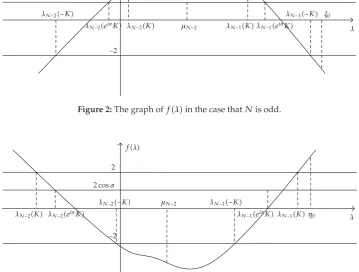
λN−2−K

λN−2eiαK

2 cosα

−2 2

fλ

λN−2K μN−2 λN−1K λN−1eiαK

λN−1−K ξ0

λ

Figure 2:The graph offλ in the case thatNis odd.

λN−2K λN−2eiαK

2 cosα

−2 2

fλ

λN−2−K μN−2 λN−1−K

λN−1eiαK λN−1K η0 _λ

Figure 3:The graph offλ in the case thatNis even.

any two consecutive eigenvalues of the separated boundary value problem1.1 with2.7 . Hence, 1.1 and 1.2 with α 0; α /0, −π < α < π; α πhas only one eigenvalue between any two consecutive eigenvalues of 1.1 with 2.7 , respectively. In addition, by Proposition 3.6, iffμk 2 or−2 andfμk 0, thenμkis not only an eigenvalue of1.1 with2.7 but also a multiple eigenvalue of1.1 and1.2 withα0 andαπ.

By Proposition 3.5i , ifN is odd, fμN−2 ≥ 2 and ifN is even, fμN−2 ≤ −2. It

follows3.22 that ifNis odd, thenfλ → −∞asλ → ∞,and ifNis even, thenfλ →

∞asλ → ∞. Hence, ifNis odd, then there exists a constantξ0> μN−2such thatfξ0 ≤ −2,

which, together withProposition 3.6, implies that1.1 and1.2 withα0;α /0,−π < α < π;

απ,has only one eigenvalueλN−1K ,λN−1eiαK , andλN−1−K , satisfying

μN−2≤λN−1K < λN−1

eiα_K_{< λ}

N−1−K ≤ξ0 3.46

seeFigure 2. Similarly, in the other case that Nis even, there exists a constantη0 > μN−2

(17)

α0;α /0,−π < α < π;απhas only one eigenvalueλN−1K ,λN−1eiαK , andλN−1−K ,

satisfying

μN−2≤λN−1−K < λN−1

eiαK< λN−1K ≤η0 3.47

seeFigure 3 . Therefore, we get that1.1 and1.2 withα /0,−π < α < π,hasNeigenvalues and it is real and satisfies

ν0≤λ0K < λ0

eiαK< λ0−K ≤μ0≤λ1−K < λ1

eiαK< λ1K ≤μ1

≤λ2K < λ2

eiαK< λ2−K ≤μ2≤λ3−K < λ3

≤ · · · ≤μN−3≤λN−2−K < λN−2

eiαK< λN−2K ≤μN−2≤λN−1K

< λN−1

eiαK< λN−1−K ≤ξ0, ifN is odd,

ν0≤λ0K < λ0

eiαK< λ0−K ≤μ0≤λ1−K < λ1

≤λ2K < λ2

eiα_K_{< λ}

2−K ≤μ2≤λ3−K < λ3

eiα_K_{< λ}

3K ≤μ3

≤ · · · ≤μN−3≤λN−2K < λN−2

eiαK< λN−2−K ≤μN−2≤λN−1−K

< λN−1

eiαK< λN−1K ≤η0, ifN is even.

3.48

This completes the proof.

Remark 3.9. LetK I, that is,k11 k22 1,k12 k21 0. Thenfλ ϕN−1λ ψNλ . In this case, Propositions3.5and3.8are the same as those mentioned in4, Propositions 3.1, 3.3–3.5, respectively, and most of the results ofProposition 3.6are the same as the results of

4, Proposition 3.2.

Acknowledgments

Many thanks to Johnny Hendersonthe editor and the anonymous reviewers for helpful comments and suggestions. This research was supported by the Natural Scientific Foundation of Shandong Province Grant Y2007A27 , Grant Y2008A28 , and the Fund of Doctoral Program Research of University of JinanB0621 .

References

1 F. V. Atkinson, Discrete and Continuous Boundary Problems, vol. 8 of Mathematics in Science and Engineering, Academic Press, New York, NY, USA, 1964.

2 Y. Shi and S. Chen, “Spectral theory of second-order vector diﬀerence equations,” Journal of Mathematical Analysis and Applications, vol. 239, no. 2, pp. 195–212, 1999.

(18)

4 Y. Wang and Y. Shi, “Eigenvalues of second-order diﬀerence equations with periodic and antiperiodic boundary conditions,”Journal of Mathematical Analysis and Applications, vol. 309, no. 1, pp. 56–69, 2005.

5 E. A. Coddington and N. Levinson,Theory of Ordinary Diﬀerential Equations, McGraw-Hill, New York, NY, USA, 1955.

6 J. K. Hale,Ordinary Diﬀerential Equations, vol. 20 ofPure and Applied Mathematics, Wiley-Interscience, New York, NY, USA, 1969.

7 W. Magnus and S. Winkler,Hill’s Equation, Interscience Tracts in Pure and Applied Mathematics, no. 20, Wiley-Interscience, New York, NY, USA, 1966.

8 M. Zhang, “The rotation number approach to eigenvalues of the one-dimensionalp-Laplacian with periodic potentials,”Journal of the London Mathematical Society, vol. 64, no. 1, pp. 125–143, 2001.

9 R. P. Agarwal, M. Bohner, and P. J. Y. Wong, “Sturm-Liouville eigenvalue problems on time scales,”