Dynamics of a delayed worm propagation model with quarantine

R E S E A R C H

Open Access

Dynamics of a delayed worm propagation

model with quarantine

Zizhen Zhang

_{and Limin Song}

*_{Correspondence:}

[email protected]

1_{School of Management Science}

and Engineering, Anhui University of Finance and Economics, Bengbu, 233030, China

Full list of author information is available at the end of the article

Abstract

A delayed SEIQRS-V model with quarantine describing the dynamics of worm propagation is considered in the present paper. Local stability of the endemic equilibrium is addressed and the existence of a Hopf bifurcation at the endemic equilibrium is established by analyzing the corresponding characteristic equation. By means of the normal form theory and the center manifold theorem, properties of the Hopf bifurcation at the endemic equilibrium are investigated. Finally, numerical simulations are also given to support our theoretical conclusions.

Keywords: SEIQRS-V model; worms; Hopf bifurcation; periodic solutions

1 Introduction

A computer worm is a self-contained program that can spread functional copies of it-self or its segments to other systems without depending on another program to host its code [, ]. With the development of information technology and the increase of network complexity, the problem of computer worms has become the focus with its tremendous destruction. So, it is of considerable interest to understand the law governing spread of the worms in a network. Enlightened by the fact that propagation of the worms in a network could be compared with infectious diseases in a population, many mathematical models have been established to predict the spread of worms [–].

The quarantine strategy is an effective method on controlling disease. Inspired of this, many researchers introduce the quarantine strategy into mathematical models to inves-tigate the spread of the worms in a network [–]. In order to describe the dynamics of worm propagation in a network, Kumaret al.proposed the following SEIQRS-V model in []:

⎧ ⎪ ⎪ ⎪ ⎪ ⎪ ⎪ ⎪ ⎪ ⎪ ⎪ ⎪ ⎨ ⎪ ⎪ ⎪ ⎪ ⎪ ⎪ ⎪ ⎪ ⎪ ⎪ ⎪ ⎩

dS(t)

dt =A–βS(t)I(t) –dS(t) –ρS(t) +θR(t) +χV(t), dE(t)

dt =βS(t)I(t) –dE(t) –γE(t), dI(t)

dt =γE(t) –dI(t) –αI(t) –δI(t) –ηI(t), dQ(t)

dt =δI(t) –dQ(t) –αQ(t) –εQ(t), dR(t)

dt =εQ(t) –dR(t) –θR(t) +ηI(t), dV(t)

dt =ρS(t) –dV(t) –χV(t),

()

where S(t),E(t),I(t), Q(t), R(t) andV(t) are the numbers of the uninfected computers which have no immunity, the exposed computers which are susceptible to infection, the in-fected computers which have to be cured, the inin-fected computers which are quarantined, the uninfected computers which have temporary immunity and the vaccinated computers which have susceptibility to infection at timet, respectively.Ais the rate at which the new computers are attached to the network;dis the natural death rate of the computers in the network;αis the death rate of computers in the network due to the attack of the worms;

β,γ,δ,η,ε,θ,ρandχare the state transition rates of system ().

Clearly, system () neglects the delays during the propagation process of the worms in the network. It is well known that delays of one type or another have been incorpo-rated into worm propagation models due to latent period, temporary immunization pe-riod or other reasons. Worm propagation models with delay have been investigated by some scholars at home or broad in recent years [–]. Delays can play a complicated role in the dynamics of the dynamical models, especially they can cause Hopf bifurcation in the predator-prey models [–], epidemic models [–] and economic models [– ]. For worm propagation models, the occurrence of a Hopf bifurcation means that the state of the worm propagation changes from an equilibrium to a limit cycle and this phe-nomenon makes the propagation of worms out of control. Therefore, it is of substantial importance to investigate the effect of delays on the worm propagation models. Based on this and considering the fact that one of the typical features of worms is its latent charac-teristic, we incorporate the latent period delay into system () and get the following worm propagation model with quarantine strategy and time delay:

⎧ ⎪ ⎪ ⎪ ⎪ ⎪ ⎪ ⎪ ⎪ ⎪ ⎪ ⎪ ⎨ ⎪ ⎪ ⎪ ⎪ ⎪ ⎪ ⎪ ⎪ ⎪ ⎪ ⎪ ⎩

dS(t)

dt =A–βS(t)I(t) –dS(t) –ρS(t) +θR(t) +χV(t), dE(t)

dt =βS(t)I(t) –dE(t) –γE(t–τ), dI(t)

dt =γE(t–τ) –dI(t) –αI(t) –δI(t) –ηI(t), dQ(t)

dt =δI(t) –dQ(t) –αQ(t) –εQ(t), dR(t)

dt =εQ(t) –dR(t) –θR(t) +ηI(t), dV(t)

dt =ρS(t) –dV(t) –χV(t),

()

whereτ is the latent period delay.

The rest of the present paper is organized as follows. In Section , we analyze the local stability of the endemic equilibrium and the threshold of a Hopf bifurcation. Section  is devoted to the explicit formulas determining direction of the Hopf bifurcation and stability of the bifurcating periodic solutions. In Section , a simulation example is presented and the simulation results match well with our obtained theoretical results. Finally, Section  draws the conclusions.

2 Analysis of Hopf bifurcation

By a direct computation, we can know that if AR(d+χ) >d + (ρ+χ)d andβ(d+

θ)(d+α+ε) >Rθ εδ+Rθ η(d+α+ε), then system () has a unique endemic

equilib-riumP∗(S∗,E∗,I∗,Q∗,R∗,V∗), where

S∗=(d+γ)(d+α+δ+η)

βγ =



R

, E∗=d+α+δ+η

R∗= εδ+η(d+α+ε)

(d+θ)(d+α+ε)I∗, V∗=

ρ

(d+χ)R

,

Q∗= δ

d+α+εI∗, I∗=

(d+θ)(d+α+ε)[d_{+ (ρ+χ)d–AR}

(d+χ)]

(d+χ)[Rθ εδ+ (d+α+ε)(Rθ η–βd–βθ)]

,

R=

βγ

(d+γ)(d+α+δ+η).

The linearized system of system () atP∗(S∗,E∗,I∗,Q∗,R∗,V∗) can be given by

dS(t)

dt =aS(t) +aI(t) +aR(t) +aV(t), dE(t)

dt =aS(t) +aE(t) +aI(t) +bE(t–τ), dI(t)

dt =aI(t) +bE(t–τ), dQ(t)

dt =aI(t) +adQ(t), dR(t)

dt =aI(t) +aQ(t) +aR(t), dV(t)

dt =aS(t) +aV(t).

()

The characteristic equation for system () is

λ+rλ+rλ+rλ+rλ+rλ+r

+sλ+sλ+sλ+sλ+sλ+s

e–λτ = , ()

where

r=aaaa(aa–aa),

r=aa

aa(a+a) +aa(a+a)

–aaaa(a+a)

–aa

aa(a+a) +aa(a+a),

r= (a+a)

aa(a+a) +aa(a+a)

+aa

aa+aa+ (a+a)(a+a)

–aa

aa+aa+ (a+a)(a+a)

+aaaa,

r=aa(a+a+a+a) –aa(a+a+a+a)

–aa(a+a) +aa(a+a)

– (a+a)

aa+aa+ (a+a)(a+a),

r=aa+aa+aa–aa– (a+a)(a+a)

r= –(a+a+a+a+a+a),

s=aaaab(a–a) +aaab(aa–aa)

+aaaa(ab–ab),

s=ab

aa(a+a) +aa(a+a)

+aaab(a+a) –aab

aa+a(a+a)

–aaaab–aaab(a+a)

+aab

aa+a(a+a) –aaaab

–ab

aa(a+a) +aa(a+a),

s=aaab+aab(a+a+a)

+aab(a+a+a) –aaab

–ab

aa+aa+ (a+a)(a+a)

+ab

aa+aa+ (a+a)(a+a)

+b

aa(a+a) +aa(a+a) ,

s=ab(a+a+a+a) +aab–aab

–b

aa+aa+ (a+a)(a+a)

–ab(a+a+a+a),

s=b(a+a+a+a+a) –ab, s= –b.

Whenτ= , equation () becomes

λ+rλ+rλ+rλ+rλ+rλ+r= , ()

with

r=r+s, r=r+s, r=r+s,

r=r+s, r=r+s, r=r+s.

Obviously,D=r> . Therefore, a set of sufficient conditions for all roots of equation

() to have a negative real part is given by the Routh-Hurwitz criteria in the following form:

D=det

r 

r r

> , ()

D=det

⎛ ⎜ ⎝

r  

r r r

r r r

⎞ ⎟

⎠> , ()

D=det

⎛ ⎜ ⎜ ⎜ ⎝

r   

r r r 

r r r r

 r r r

⎞ ⎟ ⎟ ⎟

D=det

⎛ ⎜ ⎜ ⎜ ⎜ ⎜ ⎜ ⎝

r    

r r r  

r r r r r

 r r r r

   r r

⎞ ⎟ ⎟ ⎟ ⎟ ⎟ ⎟ ⎠

> , ()

D=r> . ()

Assume thatλ=iω(ω> ) is a solution of equation (). Then one can obtain

⎧ ⎪ ⎪ ⎪ ⎪ ⎪ ⎨ ⎪ ⎪ ⎪ ⎪ ⎪ ⎩

(sω–sω+sω)sinτ ω+ (sω–sω+s)cosτ ω

=ω_–r

ω+rω–r,

(sω–sω+sω)cosτ ω– (sω–sω+s)sinτ ω

=rω–rω–rω,

()

from which it follows that

ω+pω+pω+pω+pω+pω+p= , ()

where

p=r–s, p=r– rr–s+ ss,

p=r+ rr– rr+ ss–s– ss,

p=r+ rr– r– rr–s– ss+ ss,

p=r+ r– rr+ ss–s, p=r–s– r.

If all the coefficients of system () are given, we can solve equation () by Matlab soft-ware package easily. So, we make the following assumption.

(H) equation () has at least one positive root.

If the condition (H) holds, then there existsω>  such that equation () has a pair of

purely imaginary roots±iω. Forω, one can obtain

τ=



ω×

arccos

F(ω)

F(ω)

, ()

where

F(ω) = (s–sr)ω+ (sr+sr–sr–s)ω

+ (sr+sr–sr–sr–sr+s)ω

+ (sr+sr–sr–sr–sr)ω

+ (sr+sr+sr)ω–sr,

F(ω) =sω +

s_– ss

ω_+s_+ ss– ss

ω_

+s_+ ss– ss

ω_+s_– ss

For equation (), by direct computation we have

dλ dτ =

G(λ)

H(λ), ()

where

G(λ) =λsλ+sλ+sλ+sλ+sλ+s

e–λτ_, H(λ) = λ+ rλ+ rλ+ rλ+ rλ+r

+sλ+ sλ+ sλ+ sλ+s

e–λτ

–τsλ+sλ+sλ+sλ+sλ+s

e–λτ_.

Then we obtain

dλ dτ

–

= – λ

_{+ r}

λ+ rλ+ rλ+ rλ+r

λ(λ_+r

λ+rλ+rλ+rλ+rλ+r)

+ sλ

_{+ s}

λ+ sλ+ sλ+s

λ(sλ+sλ+sλ+sλ+sλ+s)

–τ

λ. ()

Thus,

Re

dλ dτ

–

τ=τ

= f

_(v∗)

(sω–sω+sω)+ (sω–s– ω+s)

, ()

withf(v) =v_+p

v+pv+pv+pv+pv+pandv∗=ω.

Therefore, if we have the condition (H):f(v∗)= , thenRe[dλ/dτ]–τ=τ= . Accord-ing to the discussion above and the Hopf bifurcation theorem in [], we can obtain the following.

Theorem  For system(),if the conditions(H)-(H)hold,then the endemic equilibrium

P∗(S∗,E∗,I∗,Q∗,R∗,V∗)is asymptotically stable forτ ∈[,τ);a Hopf bifurcation occurs

at the endemic equilibrium P∗(S∗,E∗,I∗,Q∗,R∗,V∗)whenτ =τand a family of periodic

solutions bifurcate from the endemic equilibrium P∗(S∗,E∗,I∗,Q∗,R∗,V∗)nearτ=τ.

3 Direction and stability of the Hopf bifurcation

Motivated by the ideas of Hassardet al.[], in this section, we will derive the explicit formulas that determine the direction and stability of the Hopf bifurcation at the critical valueτ. For the sake of simplicity, letτ=τ+μ,μ∈R. Thenμ=  is the Hopf bifurcation

value for system (). Settingu(t) =S(t) –S∗,u(t) =E(t) –E∗,u(t) =I(t) –I∗,u(t) =Q(t) –

Q∗,u(t) =R(t) –R∗,u(t) =V(t) –V∗andt→(t/τ). Then system () can be transformed

into functional differential equations inC=C([–, ],R):

˙

u(t) =Lμut+f(μ,ut), ()

with

Lμφ= (τ+μ)

Bφ() +Bφ(–)

f(μ,φ) = (τ+μ)

Based on the Riesz representation theorem, there exists a bounded variation function

η(θ,μ) forθ∈[–, ] such that

Then system () can be transformed into

˙

u(t) =A(μ)ut+R(μ)ut, ()

In order to construct the coordinates describing the center manifold nearμ= , we have

In addition, from equation (), one can get the expression ofM¯:

W(θ) = –

Then we can get the following coefficients:

C() =

Thus, the properties of the Hopf bifurcation of system () can be stated as follows.

Theorem  μdetermines the direction of the Hopf bifurcation:ifμ>  (μ< ),then the

Hopf bifurcation is supercritical(subcritical);ρdetermines the stability of the bifurcating

periodic solutions:ifρ<  (ρ> ),then the bifurcating periodic solutions are stable(

un-stable);Tdetermines the period of the bifurcating periodic solutions:if T>  (T< ),

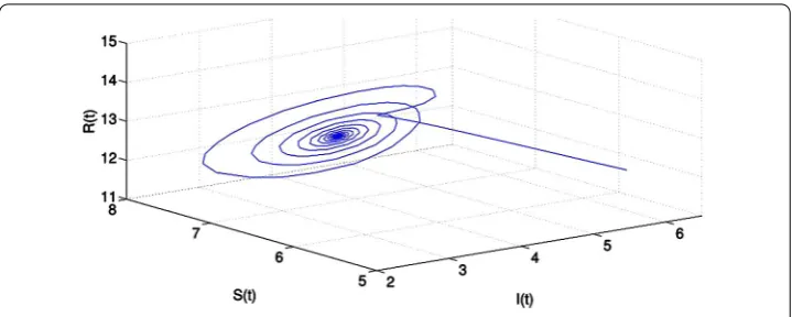
Figure 1 The phase plot of the statesS,I,Rforτ= 9.28 < 9.7698 =τ0.

4 Numerical simulation

This section is concerned with some numerical simulations of system () with the aim of verifying the obtained theoretical results. We chooseA= ,β= .,d= .,ρ= .,

θ = .,χ= .,γ = .,α= .,δ= .,η= . andε= .. Then system () becomes

⎧ ⎪ ⎪ ⎪ ⎪ ⎪ ⎪ ⎪ ⎪ ⎪ ⎪ ⎪ ⎨ ⎪ ⎪ ⎪ ⎪ ⎪ ⎪ ⎪ ⎪ ⎪ ⎪ ⎪ ⎩

dS(t)

dt =  – .S(t)I(t) – .S(t) – .S(t) + .R(t) + .V(t), dE(t)

dt = .S(t)I(t) – .E(t) – .E(t–τ), dI(t)

dt = .E(t–τ) – .I(t) – .I(t) – .I(t) – .I(t), dQ(t)

dt = .I(t) – .Q(t) – .Q(t) – .Q(t), dR(t)

dt = .Q(t) – .R(t) – .R(t) + .I(t), dV(t)

dt = .S(t) – .V(t) – .V(t).

()

It is easy to verify thatR= .,AR(d+χ) = .,d+ (ρ+χ)d= .,β(d+

θ)(d+α+ε) = .. Therefore,AR(d+χ) >d+ (ρ+χ)dandβ(d+θ)(d+α+ε) >

Rθ εδ+Rθ η(d+α+ε) is satisfied. Then one can obtain the unique endemic equilibrium

P∗(., ., ., ., ., .) of system (). It can be verified that the conditions for the occurrence of a Hopf bifurcation are also satisfied for system ().

Then, using Matlab . software package and by some complicated computations, we obtain ω= ., τ= .,λ(τ) = . – .i. We chooseτ = . <τ=

.. Thus, the endemic equilibriumP∗(., ., ., ., ., .) is asymptotically stable when τ <τ, which can be illustrated by computer simulations

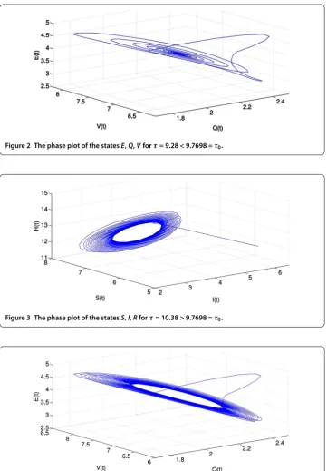
in Figures -. Whenτpasses through the critical valueτ= ., the endemic

equilib-riumP∗(., ., ., ., ., .) loses its stability and a Hopf bifur-cation occurs,i.e., a family of periodic solutions bifurcate from the endemic equilibrium

P∗(., ., ., ., ., .). Choosingτ= . >τ= ., the

computer simulations are as shown in Figures -.

Further, we haveC() = –. – .i,μ= . > ,β= –. <  andT=

. > . Therefore, according to Theorem , the Hopf bifurcation at the critical value

τ= . is supercritical; the bifurcating periodic solutions are stable and the period of

Figure 2 The phase plot of the statesE,Q,Vforτ= 9.28 < 9.7698 =τ0.

Figure 3 The phase plot of the statesS,I,Rforτ= 10.38 > 9.7698 =τ0.

Figure 4 The phase plot of the statesE,Q,Vforτ= 10.38 > 9.7698 =τ0.

5 Conclusions

We obtained the sufficient conditions for the local stability of the endemic equilibrium. The stability criteria in the absence of the delay are no longer enough to guarantee the stability in the presence of the delay, rather there is a critical valueτsuch that the model

is stable forτ <τand become unstable forτ >τ. By choosing the latent period delay

as a bifurcation parameter, and analyzing the corresponding characteristic equation, it is proved that the latent period delay in the model can destabilize the endemic equilibrium and give rise to a Hopf bifurcation. That is, a family of periodic solutions bifurcate from the endemic equilibrium when the delay passes through the critical value. Therefore, we can conclude that when the value of the latent period delay is suitable small, it is helpful to predict and control the propagation of the worms in system (). Otherwise, the worms persist in the whole host population. For further research, properties of the Hopf bifurca-tion such as direcbifurca-tion and stability are determined by applying the normal theory and the center manifold theorem. Finally, the results are validated by some numerical simulations. It should be pointed out that many other factors besides time delay can influence a worm propagation system in a real network environment. For example, network congestion and the network topology are also impact factors to worm propagation. Namely, we will link the results obtained with the model proposed in the present paper with the results coming from the networks theory. They will be a major emphasis of our future research.

Acknowledgements

This research was supported by Natural Science Foundation of Anhui Province (Nos. 1608085QF145, 1608085QF151, 1708085MA17) and Natural Science Foundation of the Higher Education Institutions of Anhui Province (No. KJ2015A144).

Competing interests

The authors declare that they have no competing interests.

Authors’ contributions

All authors contributed equally to the writing of this paper. All authors read and approved the final manuscript.

Author details

1_{School of Management Science and Engineering, Anhui University of Finance and Economics, Bengbu, 233030, China.} 2_{Department of Computer, Liaocheng College of Education, Liaocheng, 252004, China.}

Publisher’s Note

Springer Nature remains neutral with regard to jurisdictional claims in published maps and institutional affiliations.

Received: 17 March 2017 Accepted: 17 May 2017

References

1. Kumar, M, Mishra, BK, Panda, TC: Predator-prey models on interaction between computer worms, Trojan horse and antivirus software inside a computer system. Int. J. Secur. Appl.10, 173-190 (2016)

2. Mishra, BK, Pandey, SK: Dynamic model of worms with vertical transmission in computer network. Appl. Math. Comput.217, 8438-8446 (2011)

3. Toutonji, OA, Yoo, SM, Park, M: Stability analysis of veisv propagation modeling for network worm attack. Appl. Math. Model.36, 2751-2761 (2012)

4. Peng, S, Wu, M, Wang, G, et al.: Propagation model of smartphone worms based on semi-Markov process and social relationship graph. Comput. Secur.44, 92-103 (2014)

5. Mishra, BK, Keshri, N: Mathematical model on the transmission of worms in wireless sensor network. Appl. Math. Model.37, 4103-4111 (2013)

6. Mishra, BK, Pandey, SK: Dynamic model of worm propagation in computer network. Appl. Math. Model.38, 2173-2179 (2014)

7. Mishra, BK, Pandey, SK: Fuzzy epidemic model for the transmission of worms in computer network. Nonlinear Anal., Real World Appl.11, 4335-4341 (2010)

8. Wang, FW, Yang, Y, Zhao, DM, et al.: A worm defending model with partial immunization and its stability analysis. J. Commun.10, 276-283 (2015)

9. Wang, F, Zhang, Y, Wang, C, et al.: Stability analysis of a SEIQV epidemic model for rapid spreading worms. Comput. Secur.29, 410-418 (2010)

11. Yao, Y, Zhang, N, Xiang, WL, et al.: Modeling and analysis of bifurcation in a delayed worm propagation model. J. Appl. Math.2013, Article ID 927369 (2013)

12. Wang, C, Chai, S: Hopf bifurcation of an SEIRS epidemic model with delays and vertical transmission in network. Adv. Differ. Equ.2016, 100 (2016)

13. Yao, Y, Xiang, WL, Qu, AD,et al.: Hopf bifurcation in an SEIDQV worm propagation model with quarantine strategy. Discrete Dyn. Nat. Soc.2012, Article ID 304868 (2012)

14. Yao, Y, Feng, X, Yang, W,et al.: Analysis of a delayed Internet worm propagation model with impulsive quarantine strategy. Math. Probl. Eng.2014, Article ID 369360 (2014)

15. Zhang, ZZ, Yang, HZ: Stability and Hopf bifurcation in a delayed SEIRS worm model in computer network. Math. Probl. Eng.2013, Article ID 319174 (2013)

16. Liu, J: Bifurcation analysis of a delayed predator-prey system with stage structure and Holling-II functional response. Adv. Differ. Equ.2015, 208 (2015)

17. Wang, LS, Feng, GH: Global stability of an eco-epidemiological predator-prey model with saturation incidence. J. Appl. Math. Comput.53, 303-319 (2017)

18. Pal, N, Samanta, S, Biswas, S, et al.: Stability and bifurcation analysis of a three-species food chain model with delay. Int. J. Bifurc. Chaos25, 1550123 (2015)

19. Biswas, S, Sasmal, SK, Samanta, S, et al.: Optimal harvesting and complex dynamics in a delayed eco-epidemiological model with weak Allee effects. Nonlinear Dyn.87, 1553-1573 (2017)

20. Liu, J, Wang, K: Hopf bifurcation of a delayed SIQR epidemic model with constant input and nonlinear incidence rate. Adv. Differ. Equ.2016, 168 (2016)

21. Wang, WY, Chen, LJ: Stability and Hopf bifurcation analysis of an epidemic model by using the method of multiple scales. Math. Probl. Eng.2016, Article ID 2034136 (2016)

22. Sun, XG, Wei, JJ: Stability and bifurcation analysis in a viral infection model with delays. Adv. Differ. Equ.2015, 332 (2015)

23. Wang, TL, Hu, ZX, Liao, FC: Stability and Hopf bifurcation for a virus infection model with delayed humoral immunity response. J. Math. Anal. Appl.411, 63-74 (2014)

24. Liu, J: Bifurcation of a delayed SEIS epidemic model with a changing delitescence and nonlinear incidence rate. Discrete Dyn. Nat. Soc.2017, Article ID 2340549 (2017)

25. Gori, L, Guerrini, L, Sodini, M: Hopf bifurcation in a cobweb model with discrete time delays. Discrete Dyn. Nat. Soc.

2014, Article ID 137090 (2014)

26. Gori, L, Guerrini, L, Sodini, M: Hopf bifurcation and stability crossing curves in a cobweb model with heterogeneous producers and time delays. Nonlinear Anal. Hybrid Syst.18, 117-133 (2015)

27. Liao, MX, Xu, CJ, Tang, XH: Stability and Hopf bifurcation for a competition and cooperation model of two enterprises with delay. Commun. Nonlinear Sci. Numer. Simul.19, 3845-3856 (2014)

28. Hassard, BD, Kazarinoff, ND, Wan, YH: Theory and Applications of Hopf Bifurcation. Cambridge University Press, Cambridge (1981)

29. Bianca, C, Ferrara, M, Guerrini, L: The time delays’ effects on the qualitative behavior of an economic growth model. Abstr. Appl. Anal.2013, Article ID 901014 (2013)

30. Bianca, C, Ferrara, M, Guerrini, L: The Cai model with time delay: existence of periodic solutions and asymptotic analysis. Appl. Math. Inf. Sci.7, 21-27 (2013)

31. Meng, XY, Huo, HF, Zhang, XB, et al.: Stability and Hopf bifurcation in a three-species system with feedback delays. Nonlinear Dyn.64, 349-364 (2011)

32. Jana, D, Agrawal, R, Upadhyay, RK: Top-predator interference and gestation delay as determinants of the dynamics of a realistic model food chain. Chaos Solitons Fractals69, 50-63 (2014)