Various breathers and rogue waves for the coupled long wave short wave system

(1)

R E S E A R C H

Open Access

Various breathers and rogue waves for the

coupled long-wave-short-wave system

Chuanjian Wang

1*

_{and Zhengde Dai}

2

*_{Correspondence:}

wcj20082002@aliyun.com 1_{Department of Mathematics,}

Kunming University of Science and Technology, Kunming, Yunnan 650500, P.R. China

Full list of author information is available at the end of the article

Abstract

Explicit forms of various breathers, including inclined periodic breather, Akhmediev breather, Ma breather and rogue wave solutions, are obtained for the coupled long-wave-short-wave system by using a Hirota two-soliton method with complex frequency and complex wave number. Based on the structures of these breather solutions and ﬁgures via computer simulation, the characteristics of various breather solutions are discussed which might provide us with useful information on the dynamics of the relevant physical ﬁelds.

Keywords: coupled long-wave-short-wave system; Hirota two-soliton method; breather; rogue wave

1 Introduction

It is well known that solitary wave solutions of nonlinear evolution equations play an im-portant role in nonlinear science fields, especially in nonlinear physical science, since they can provide much physical information and more insight into the physical aspects of the problem and thus lead to further applications []. In recent years, rogue waves, as a special type of solitary waves, have triggered much interest in various physical branches. Rogue waves, alternatively called freak or giant waves, were first observed under circumstances of arbitrary depths of the ocean. One always has two or even more times higher amplitude than their surrounding waves and generally they form in a short time for which reason people think that it comes from nowhere [, ]. Rogue waves have been the subject of intensive research in oceanography [], superfluid helium [], Bose-Einstein condensates [], optical fibers [], plasma physics [], financial markets and related fields [–]. The first-order rational solution of the self-focusing nonlinear Schödinger equation (NLS) was first found by Peregrine to describe the rogue waves phenomenon []. Recently, by us-ing the Darboux dressus-ing technique or the Hirota bilinear method, rogue waves solutions in complex systems such as described by the Hirota equation, Sasa-Satsuma equation, Davey-Stewartson equation, coupled Gross-Pitaevskii equation, coupled NLS Maxwell-Bloch equation and so on have been demonstrated [–].

Now we consider the following coupled long-wave-short-wave system [–]:

⎧ ⎪ ⎨ ⎪ ⎩

ipt– pxx+ p(b–ω) = ,

iqt– qxx+ q(b–ω) = ,

bt– (pq∗+p∗q)x= .

(.)

(2)

In the above equation,p(x,t) andq(x,t) are the orthogonal components of the envelope of a rapidly varying complex field (the short-wave) representing a transverse wave whose group velocity resonates with the phase velocity of a real fieldb(x,t) (the long wave) repre-senting a longitudinal wave. The∗denotes complex conjugation andωis an arbitrary real constant. The CLS equations (.) generalize the scalar long-wave-short-wave resonance equations derived by Djordjevic and Redekopp [] for long-wave-short-wave interactions when the more generic nonlinear Schrödinger equation breaks down due to a singularity in the coefficient of the cubic nonlinearity; the dispersion of the short-wave is balanced by the nonlinear interaction of the long wave, while the self-interaction of the short-wave drives the evolution of the long wave. Other studies of long-wave-short-wave interactions include those by Benney [] and Grimshaw []. The CLS equations (.) are integrable in the sense that they possess an equivalent scattering problem formulation as a Lax pair of commuting differential operators on a subalgebra ofsl(). Wright III [] has obtained an auto-Bäklund transformation for plane-wave solutions of a system of coupled long-wave-short-wave equations by using the dressing method. The spatially periodic orbits on a homoclinic manifold of a torus of spatially independent plane waves were constructed by evaluating the auto-Bäklund transformation.

2 Hirota two-soliton method and various breathers

In this section, we will use the Hirota two-soliton method [, ] to construct our result.

2.1 Hirota two-soliton method

Hirota two-soliton method was ﬁrst proposed by Hirota []. For a general nonlinear par-tial diﬀerenpar-tial equation in the formP(u,ut,ux, . . .) = ,Pis a polynomial in its arguments. By Painlevé analysis, a transformationu=T(f) is made for some new and unknown func-tionf. By using the above transformation, the original equation can be converted into Hirota’s bilinear form,

G(Dt,Dx;f) = ,

where theD-operator is deﬁned by []

Dn_tDm_xf(x,y)·g(x,t) =

∂ ∂t–

∂ ∂t

n_∂

∂x–

∂ ∂x

m

f(x,t)g x,t|x=x,t=t.

So the solutions of original partial differential equation can be converted into the solutions of bilinear differential equations. We solve the above bilinear differential equations to get breather wave solutions by using a two-soliton method with the help of MAPLE.

Now we make the dependent variable transformation [, ] for the system (.):

p=G

F, q= H

F, b=b– (lnF)xx, (.)

whereG,H are complex valued functions,F is a real valued function, andb is a

(3)

equations forF,G, andH:

linearized. Then the solutions of the system (.) can be converted into the solutions of coupled bilinear diﬀerential equations (.).

The two-soliton solutions of bilinear diﬀerential equations can be expressed in the form

⎧

exp-function algorithm [], one concludes that they are the same.

In order to obtain the required breather solutions, we consider the case thatai,ci(i= , ) are complex numbers, that is, taking wave numbers and frequencies that are complex, respectively. Indeed, leta=k–ik,a=k+ik,c=l–il,c=l+il, substituting (.)

into (.), we can obtain various breathers by restricting the parameters suitably. They can be rewritten in terms of trigonometric and hyperbolic functions. In the following, we report the explicit forms of these breather solutions.

2.2 Various breathers of the coupled long-wave-short-wave system

.. Inclined periodic breather

(4)

= k_k_l+ kkl+ k+ l

lk+ kkl

+ k_+ l_lkk+ l+ k

lk,

δ=δ, δ=δ,

whereζ =kx+lt,η=kx+lt,d= √

M(k

–k),d=  √

Mkk,d=Mk–k,φ=

ln√M,φ=ln|δ|,θ=arctan

(kkl–lk+lk)

(k

+k)–l–l .

Obviously, the parametersδ,δhave the following relation:

δδ∗= .

Some asymptotic behaviors of the obtained solutions can be found. Without loss of gen-erality, we assume thatl>  ork> , and we obtain from (.)

(p,q,b)→ pe–i(at–θ),qe–i(at–θ),b

, astorx→+∞,

and

(p,q,b)→ pe–iat,qe–iat,b

, astorx→–∞.

Obviously, the limit solution (pe–i(at–θ),qe–i(at–θ),b) is an exact plane-wave solution of

(.). This means that in some limit,t→ ±∞orx→ ±∞or in both, this new solution will approach the original plane-wave solution, up to some phase shift. It is shown that this solution, given by (.), represents a kind of homoclinic solution and meanwhile contains a periodic wavecosξ whose amplitude periodically oscillates with the evolution of time. So this solution represented by (p,q,b) of (.) is a homoclinic breather solution. The trajectory of these solutions is deﬁned explicitly by

x= –lt+φ+r

k

,

which can be derived fromζ +φ+r= . So the solution in (.) evolves periodically

(5)

Figure 1 Inclined periodic breather proﬁles of|p(x,t)|2_{(a) and}_b₍_x_,_t_{) (b).}_{The parameters are selected as}

k2=l2= 0.2,p0= 0.5,q0= 0.4,a= 1,b0= –1. A similar proﬁle occurs forqalso (not shown here). Curved lines drawn at the bottom of this ﬁgure are contour lines.

t→–∞, which is diﬀerent. In this case, this solution is a heteroclinic breather solution. In fact, this solution is called a complexiton solution in Ref. [].

From the inclined periodic breather solution we can derive the Akhmediev breather [] (space periodic breather solution), Ma breather [] (time periodic breather solution) and

rogue wave solutions.

.. Ma breather

To obtain the Ma breather solution, we consider the choicel=  in (.). In this case,

ζ =  implies that the trajectory equation of these solutions can be expressed asx= . So

(6)

Figure 2 Ma breather proﬁles of|p(x,t)|2(a) andb(x,t) (b).The parameters are selected ask2= 0.1,

p0=a=b0= 1,q0= 0.04. A similar proﬁle occurs for|q|2also (not shown here). Curved lines drawn at the bottom of this ﬁgure are contour lines.

the straight line with thex-axis, that is,

⎧ ⎪ ⎪ ⎪ ⎨ ⎪ ⎪ ⎪ ⎩

p=pe–i(at+θ)

√

Mcosh_√ (kx+φ+iθ)+cos((kx+lt)–iφ) Mcosh(kx+φ)+cos(kx+lt) ,

q=qe–i(at+θ)

√

Mcosh_√ (kx+φ+iθ)+cos((kx+lt)–iφ) Mcosh(kx+φ)+cos(kx+lt) ,

b=b–(dcosh(kx+₍φ√)cos_M_cosh(kx₍+_klt)+dsinh(kx+φ)sin(kx+lt)+d)

x+φ)+cos(kx+lt)) ,

(.)

whereφ=φ+r. This solution tends to the plane-wave solution asx→ ∞. We depict this

solution (.) in Figure . The plot shows that this solution is periodic with periodπ l int and localized, exponentially decaying in thexdirection. This solution which is temporally breathing and spatially oscillating is called a Ma breather.

.. Akhmediev breather

To obtain the Akhmediev breather solution, we consider the choicek=  in (.). In this

(7)

Figure 3 Akhmediev breather proﬁles of|p(x,t)|2_{(a) and}_b₍_x_,_t_{) (b).}_{The parameters are selected as}

l2= 0.1,p0=a=b0= 1,q0= 0.04. A similar proﬁle occurs for|q|2also (not shown here). Curved lines drawn at the bottom of this ﬁgure are contour lines.

time direction, that is,

⎧ ⎪ ⎪ ⎪ ⎨ ⎪ ⎪ ⎪ ⎩

p=pe–i(at+θ)

√

Mcosh_√ (lt+φ+iθ)+cos((kx+lt)–iφ)

Mcosh(lt+φ)+cos(kx+lt) ,

q=qe–i(at+θ)

√

Mcosh_√ (lt+φ+iθ)+cos((kx+lt)–iφ) Mcosh(lt+φ)+cos(kx+lt) ,

b=b–(dcosh(lt+φ₍√)cos_M_cosh(kx+₍_llt)+dsinh(lt+φ)sin(kx+lt)+d)

t+φ)+cos(kx+lt)) ,

(.)

whereφ=φ+r. This solution tends to the plane-wave solution ast→ ∞. In this case,

we ﬁndM=  +k

l . Therefore we see that (.) has no poles and should be well behaved everywhere. So the solution (.) is a nonsingular solution. We have plotted the solution (.) in Figure . This solution is periodic with period π

(8)

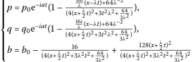
.. Rogue wave

To obtain a rogue wave from an inclined periodic breather, we consider the limit of the inclined periodic breather solution with the choicel=kλ,l= –kλ,k = k,er= –.

The propagation speed of the inclined periodic breather is given byλ. Substituting the above expressions into the inclined periodic breather form, (.) and rogue waves of the coupled long-wave-short-wave system are derived when the periods of the periodic rogue wave go to inﬁnite. Indeed, by lettingk→ in (.), (.) becomes a rational solution

⎧

This solution is nothing but the rogue wave solution of a coupled long-wave-short-wave system which is localized both in space and time. The typical spatial-temporal structure of the rogue wave is shown in Figure . From (.), the denominators of this family of so-lution are clearly nonsingular. This soso-lution is well behaved everywhere. The maximum amplitude of the rogue wave solution|p| occurs at the point (, ) and the maximum amplitude of this rogue wave solution is equal to p

. The minimum amplitude of|p|

oc-λ ), and the minimum amplitude of this rogue wave solution is equal to . A similar result occurs for|q|_{(not shown here). The maximum}

am-plitude of the rogue wave solutionboccurs at two points (t= ,x=±

λ) and the maximum amplitude of this rogue wave solution is equal tob+_λ. The minimum amplitude ofb

occurs at the point (t= ,x= ), and the minimum amplitude of this rogue wave solution is equal tob–_λ. It is easy to verify that (p,q,b) is a solution of (.). Moreover, (p,q,b)

is also a rational homoclinic solution and tends to the ﬁxed cycle (pe–iat,qe–iat,b) as t→ ∞orx→ ∞. In fact, (p,q,b)→(pe–iat+iπ,qe–iat+iπ,b) whentorx→–∞, and the

cycles (pe–iat+iπ,qe–iat+iπ,b) and (pe–iat,qe–iat,b) were one and the same. This shows

that (p,q,b) is also a homoclinic rogue wave solution of a coupled long-wave-short-wave system,p,qare bright homoclinic rogue waves andbis a dark (see Figure ). Moreover, it follows from Figure  that, as time goes to±∞, this rogue wave develops a localized hump with a peak amplitude of more than three times the non-zero constant background in the intermediate times. It is shown that the rogue wave arises from the non-zero con-stant background and then disappears into the non-zero concon-stant background again. By comparing with known results [, , ], one ﬁnds that they are similar in structure. These solutions distinguish themselves in zero-amplitude points and in a tilted angle (see Figure ).

(9)

Figure 4 Rogue wave proﬁles of|p(x,t)|2(a) andb(x,t) (b).The parameters are selected as

p0=a=b0= 1,q0= 0.04. A similar proﬁle occurs for|q|2also (not shown here). Curved lines drawn at the bottom of this ﬁgure are contour lines.

by (.) reaches its minimum or maximum at point (α,β), which is a controllable center on the (x,t) plane.

3 Conclusion and discussion

(10)

Competing interests

The authors declare that they have no competing interests.

Authors’ contributions

All authors contributed equally to the manuscript and read and approved the ﬁnal manuscript.

Author details

1_{Department of Mathematics, Kunming University of Science and Technology, Kunming, Yunnan 650500, P.R. China.} 2_{School of Mathematics and Physics, Yunnan University, Kunming, Yunnan 650500, P.R. China.}

Acknowledgements

This work was supported by Chinese Natural Science Foundation Grant Nos. 11361048, 11301235, and 11261049, Yunnan Natural Science Foundation Grant No. kksy201307141.

Received: 18 November 2013 Accepted: 26 February 2014 Published:14 Mar 2014

References

1. Ablowitz, MJ, Clarkson, PA: Solitons, Nonlinear Evolution Equations and Inverse Scattering. Cambridge University Press, Cambridge (1991)

2. Kharif, C, Pelinovsky, E, Slunyaev, A: Rogue Waves in the Ocean, Observation, Theories and Modeling. Springer, New York (2009)

3. Ganshin, AN, Eﬁmov, VB, Kolmakov, GV, Mezhov-Deglin, LP, McClintock, PVE: Observation of an inverse energy cascade in developed acoustic turbulence in superﬂuid helium. Phys. Rev. Lett.101, 065303 (2008) 4. Bludov, VYu, Konotop, VV, Akhmediev, N: Matter rogue waves. Phys. Rev. A80, 033610 (2009)

5. Montina, A, Bortolozzo, U, Residori, S, Arecchi, FT: Non-Gaussian statistics and extreme waves in a nonlinear optical cavity. Phys. Rev. Lett.103, 173901 (2009)

6. Bailung, H, Sharma, SK, Nakamura, Y: Observation of Peregrine solitons in a multicomponent plasma with negative ions. Phys. Rev. Lett.107, 255005 (2011)

7. Yan, ZY: Financial rogue waves. Commun. Theor. Phys.5, 947 (2010)

8. Akhmediev, N, Ankiewicz, A: Solitons, Nonlinear Pulses and Beams. Chapman & Hall, London (1997) 9. Agrawal, GP: Nonlinear Fiber Optics. Academic Press, New York (2001)

10. Peregrine, DH: Water waves, nonlinear Schrödinger equations and their solutions. J. Aust. Math. Soc. Ser. B, Appl. Math

25, 16 (1983)

11. Akhmediev, N, Ankiewicz, A, Soto-Crespo, JM: Rogue waves and rational solutions of the nonlinear Schrödinger equation. Phys. Rev. E80, 026601 (2009)

12. Xu, S, He, J: The Darboux transformation of the derivative nonlinear Schrödinger equation. J. Phys. A, Math. Theor.53, 063507 (2013)

13. Tao, Y, He, J: Multisolitons, breathers, and rogue waves for the Hirota equation generated by the Darboux transformation. Phys. Rev. E85, 026601 (2012)

14. Bandelow, U, Akhmediev, N: Persistence of rogue waves in extended nonlinear Schrödinger equations: integrable Sasa-Satsuma case. Phys. Lett. A376, 1558 (2012)

15. Ohta, Y, Yang, J: Dynamics of rogue waves in the Davey-Stewartson II equation. J. Phys. A, Math. Theor.46, 105202 (2013)

16. Zhao, LC, Liu, J: Rogue-wave solutions of a three-component coupled nonlinear Schrödinger equation. Phys. Rev. E

87, 013201 (2013)

17. Zhong, WP: Wave solutions of the generalized one-dimensional Gross-Pitaevskii equation. J. Nonlinear Opt. Phys. Mater.21, 1250026 (2012)

18. Li, C, He, J, Porseizan, K: Rogue waves of the Hirota and the Maxwell-Bloch equation. Phys. Rev. E87, 012913 (2013) 19. Djordjevic, VD, Redekopp, LG: On two-dimensional packets of capillary-gravity waves. J. Fluid Mech.79, 703 (1977) 20. Benney, DJ: A general theory for interactions between short and long waves. Stud. Appl. Math.56, 81 (1977) 21. Grimshaw, RHJ: The modulation of an internal gravity-wave packet, and the resonance with the mean motion. Stud.

Appl. Math.56, 241 (1977)

22. Wright, OC: On a homoclinic manifold of a coupled long-wave-short-wave system. Commun. Nonlinear Sci. Numer. Simul.15, 2066 (2010)

23. Tajiri, M, Takeuchi, K, Arai, T: Asynchronous development of the Benjamin-Feir unstable mode. Phys. Rev. E64, 056622 (2001)

24. Tajiri, M, Arai, T: Quasi-line soliton interactions of the Davey-Stewartson I equation: on the existence of long-range interaction between two quasi-line solitons through a periodic soliton. J. Phys. A, Math. Theor.44, 235204 (2011) 25. Ma, WX, Zhu, ZN: Solving the (3 + 1)-dimensional generalized KP and BKP equations by the multiple exp-function

algorithm. Appl. Math. Comput.218, 11871 (2012)

26. Ma, WX: Complexiton solutions to integrable equations. Nonlinear Anal.63, e2461 (2005)

27. Chabchoub, A, Hoﬀmann, N, Onorato, M, Akhmediev, N: Super rogue waves: observation of a higher-order breather in water waves. Phys. Rev. E2, 011015 (2012)

28. Chabchoub, A, Hoﬀmann, NP, Akhmediev, N: Rogue wave observation in a water wave tank. Phys. Rev. E106, 204502 (2011)

29. Ma, WX: Bilinear equations and resonant solutions characterized by Bell polynomials. Rep. Math. Phys.72, 41 (2013)

10.1186/1687-1847-2014-87