R E S E A R C H
Open Access
Blind recognition of binary cyclic codes
Zhou Jing, Huang Zhiping
*, Su Shaojing and Yang Shaowu
Abstract
A solution to blind recognition of binary cyclic codes is proposed in this paper. This problem could be addressed on the context of non-cooperative communications or adaptive coding and modulations. We consider it as a reverse engineering problem of error-correcting coding. The proposed algorithm recovers the encoder parameters of a cyclic, coded communication system with the only knowledge of the noisy information streams. By taking advantages of soft-decision outputs of the channel and by employing statistical signal-processing methods, it achieves higher recognition performances than existing algorithms which are based on algebraic approaches in hard-decision situations. By comprehensive simulations, we show that the probability of false estimation of coding parameters of our proposed algorithm is much lower than the existing algorithms, and falls rapidly when signal-to-noise ratio increases.
Keywords:Blind recognition; Channel coding; Cyclic codes; Reverse engineering
1. Introduction
The blind recognition of cyclic codes is a reverse engin-eering problem of the error-correcting coding which can be applied to non-cooperative communications [1,2] and adaptive coding and modulations (ACM) [3-6]. In most cases of digital communications, forward error-correcting coding is used to protect the transmitted information against noisy channels to reduce errors which occur during transmission. Cyclic codes are one class of the most important error-correcting codes ap-plied in communication area. In cooperative context, the parameters of the codes and modulations are usually known by the transmitters and receivers both. But a re-ceiver in non-cooperative communications or a cognitive radio receiver may not know those parameters and thus cannot directly receive and decode the transmitted infor-mation on the channel. Therefore, to adapt itself to an unknown transmission context, the receiver must recognize the modulation and coding parameters blindly before processing the received data. In this paper, we de-velop an approach for blind recognition of the coding parameters of a communication system which uses bin-ary cyclic codes.
2. Related work
In [7], a Euclidean algorithm-based method is proposed to identify a 1/2-rate convolutional encoder in noiseless cases. However, it is not suitable for noisy channels. In [8], another approach is presented to identify a 1/n-rate convolutional encoder in noisy cases based on the Ex-pectation Maximization algorithm. The authors of [9,10] develop methods for blind recovery of convolutional encoder in turbo code configuration. In [6,11], a dual code method for blind identification ofk/n-rate convolu-tional codes is proposed for cognitive radio receivers. An iterative decoding-technique-based reconstruction of block code is introduced by the authors of [12] and was applied to low-density parity-check (LDPC) codes. An algebraic approach for the reconstruction of linear and convolutional codes is presented in [13]. In [14], an algorithm for blind recognition of error-correcting codes is presented by utilizing the rank properties of the re-ceived stream.
In [15], an approach for blind recognition of binary lin-ear block codes in low code-rate situations is presented. The authors propose to estimate the code length according to the code weight distribution characters of the low-rate codes and then get the generator matrix by im-proving the traditional simplification of matrices. It has a good performance in high bit error rate (BER) but is not suitable for high code rate situations. Furthermore, it re-quires a large amount of observed data. In [16] and [17], * Correspondence:[email protected]
Mechatronics Engineering and Automation Department, National University of Defense Technology, Changsha 410073, Hunan Province, People's Republic of China
the authors present a blind recognition algorithm for Bose-Chaudhuri-Hocquenghem (BCH) codes based on the Roots Information Dispersion Entropy and Roots Statistic (RIDERS). This algorithm can achieve correct recognition in both high and low code rate situations with the BER of 10−2. But it is computationally inten-sive, especially when the code length is large. The au-thors of [18] improve the algorithm proposed in [16,17] by reducing the computational complexity and making the recognition procedure faster.
Most of the previous works are concentrating on hard-decision situations, and are based on utilizing the algebraic properties of the codes in Galois fields (GF). The major drawback of them is that they have a low fault tolerance. Even if only 1 bit error occurs in a codeword, the algebraic properties of error-correcting codes will be largely destroyed. Therefore, the recog-nizers need a large amount of observed data. On the other hand, if soft information about the channel output is available, the soft-decision outputs can provide more information for the code recognition, and statistical sig-nal processing algorithms can also be employed to im-prove the recognition performance.
When statistic and artificial-intelligence-based iterative algorithms are applied to error-correcting decoding, the decoding performance is improved about 2 ~ 3 dB in soft-decision situations [19]. In [20,21], the authors introduce a MAP approach to achieve blind frame synchronization of error-correcting codes with a sparse parity-check matrix. It is also developed on Reed Solo-mon (RS) codes [22] and BCH product codes [23] and yields better performances than previous hard decision ones. In this paper, we propose an algorithm to achieve blind recognition of binary cyclic codes in soft-decision situations. Literature [4] also considers the blind recog-nition of coding parameters based on soft decisions. But in fact, its recognition procedure is semi-blind. The au-thors assume that the channel code which is used at the transmitter is unknown to the receiver, but the code is chosen from a set of possible codes which the authors call the candidate set. This set has a limited number of candidates, and is arranged beforehand by both the transmitter and the receiver. It has good performances on ACM, but is not suitable for non-cooperative cases.
To the best of our knowledge, this paper is the first pub-lication to consider the complete-blind recognition prob-lem of binary cyclic codes in soft-decision situations. The proposed algorithm in this paper is based on the RIDERS algorithm introduced in [16-18]. We improve and extend this work in order to handle soft-decision situations. To utilize the soft-decision outputs, we employ the idea of MAP-based processing method proposed in [20-23].
The remainder of this paper is organized as follows: section 3 briefly introduces the RIDERS algorithm in
hard decision situations proposed in [16-18]; section 4 presents the principle of our proposed recognition algo-rithm for binary cyclic codes in soft-decision situation; section 5 draws the general recognition procedure of the proposed algorithm; and finally, the simulation results and conclusions are given in sections 6 and 7.
3. RIDERS algorithm for blind recognition of BCH codes
3.1 Introduction of RIDERS algorithm
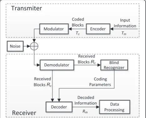
The RIDERS algorithm is introduced in [16,17] and im-proved in [18] to solve the problem of recognition of BCH codes. The system model of blind recognition problem of coding parameters is shown in Figure 1. On the transmitter, the information sequence Tm is
encoded and separated to coded blocks Tc by the
en-coder and modulated before transmitted to the chan-nel. After demodulation, the receiver blindly recognizes the coding parameters and decodes the received blocks
Rc to correct the errors which occur during the
trans-mission.Rmis the decoded information which could be
processed forward.
We define c(x) to be the codeword polynomial of Tc,
then the algebraic model of the encoding procedure can be described as follows [24]:
c xð Þ ¼m xð Þ g xð Þ ð1Þ
or in systemic form:
c xð Þ ¼m xð Þ xn−kþ m xð Þ xn−k
modg xð Þ
:
ð2Þ
wherem(x) is the input information polynomial andg(x) is the generator polynomial. The purpose of the
recognition is to estimate the codeword length and gen-erator polynomial g(x) blindly with the only knowledge of the received streams. For an encoding system,m(x) is different in each codeword, but g(x) is the same. According to Equations 1 and 2, the roots of g(x) are also the roots ofc(x). If no error occurs, the roots ofg(x) will appear in every codeword. However, for an invalid codeword, this algebraic relationship does not exist. In this paper, we define the code roots as the roots of the generator polynomial. The root space of a binary codeword polynomialc(x) defined in GF(2m) (m≥1) is a finite space, which contains 2m −1 symbols. We define
A to be the set of the generator polynomial roots. In a noisy context, statistically, for each codeword c(x), the probabilities of the codeword polynomial roots appear in
Ais larger than that inΑ (defined in GF(2m)). While for an invalid codeword polynomial c’(x), the roots of c’(x) appear randomly in GF(2m). In this case, the authors of [16-18] propose the following unproved hypothesis:
Hypothesis 1: Each symbol in GF(2m) has a uniform probability of being a root ofc’(x).
According to this hypothesis, the authors of [16-18] propose an algorithm to recognize the BCH code length by traversing all the possible code length and primitive polynomials to find the correct coding parameters that maximize the roots Information Dispersion Entropy Function (IDEF) as follows:
ΔH¼−X is a primitive element in GF(2m). pi is calculated as
follows:
pi¼Ni
N ;1≤i≤2
m−1: ð4Þ
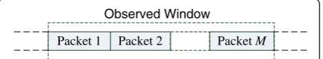
The received sequence, i.e.Rc in Figure 1, is separated
to M packets with an assumption of code length l, as shown in Figure 2. In [16-18], the authors assume that the start point of the first coding packet is obtained
according to the frame synchronization testing, while the code length and generator polynomial are unknown. We define rj(x)(1≤ j ≤ M) to be the codeword
polyno-mial of thejth packet in the received sequence. In Equa-tion 4, Ni is the times of appearances of αi being the
According to Hypothesis 1, when the estimation of code length and primitive polynomial is incorrect,
pi could be considered uniformly distributed, and pi ≈
1/(2m−1) (1 ≤i≤2m−1). Thus theΔHin Equation 2 is low. If the code parameters are estimated correctly and αi is a root of g(x), pi should be larger. Therefore,
the distribution of pi should not be uniform. Then the
information entropy ofpiis lower andΔHis larger. This
is the basic principle of estimating the code length by maximizing theΔHdefined in Equation 3.
Once the code length is estimated, by comparing piat
different roots, we can consider the obviously higher ones as the estimation of the code roots and the gener-ator polynomial could be obtained by g xð Þ ¼ðx−αi1Þ
x−αi2
ð Þ⋯ðx−αirÞ, where αi1; αi2; ⋯; αir are the
esti-mated code roots, i.e. the roots of the generator polynomial.
The RIDERS algorithm has a good performance but there are still some drawbacks which need to be im-proved, which are described as follows:
1) Hypothesis 1 proposed in [16-18] is not correct. In section 3.2, we give the proof. In fact, not all the symbols in GF(2m) have the same probability of being a root of an invalid codewordc’(x). 2) This algorithm only considers the BCH codes in
the cases of regular code length, i.e. code length l= 2m−1. The authors ignored the shortened code case, which are widely applied, however.
3) The code roots can be separated into some conjugate root groups, and each group contains several conjugate roots, which are the roots of a same minimal polynomial. If a generator polynomial g(x) has a rootβ, which is a root of the minimal polynomialmp(x), the symbols which are other roots
ofmp(x) also are part of the roots ofg(x). So we can
test which minimal polynomials are factors of the generator polynomial rather than testing which elements in GF(2m) are roots of the code. 4) This algorithm is based on the hard decision
symbols and do not utilize the soft channel outputs 5) This algorithm only considers the recognition of
BCH codes and does not discuss the applications on other binary cyclic codes.
6) The authors of [16-18] ignore the synchronization of the codewords. They assume that the starting Packet 1 Packet 2 Packet M
Observed Window
positions of the codewords have been known before the recognition procedure by framing testing. But in practical implementations, this should not be the case in blind context.
In the paragraph from section 4, we propose an im-proved RIDERS algorithm based on soft-decision situa-tions and extend the applicasitua-tions to general binary cyclic codes.
3.2 Proof of faultiness of Hypothesis 1
In this section, we present that Hypothesis 1 proposed in [16-18] is not always correct. The proof is shown below.
Proof. Let c’(x) be the codeword polynomial of a codewordC’, we can calculatepi, which is the
probabil-ity thatαiis a root ofc’(x). To calculatepi, we define the
minimal parity-check matrix Hmin(αi) corresponding to the elementαiin GF(2m) as follows:
Hmin αi ¼ αi
l−1
; αi l−2;⋯; αi 1; αi 0
: ð5Þ
We transformHmin(αi) to its binary form by replacing the symbols in Hmin (αi) by their binary column vector patterns according to the coding theory [25] and record itHbmin(αi).
For example, the minimal parity-check matrixHmin(α3) corresponding to the element α3 in GF(23) with code lengthl= 23−1 = 7 is as follows:
Hmin α3 ¼ α18 α15 ⋯ α3 1
: ð6Þ
Based on the primitive polynomial p(x) = x3 +x + 1, we can replace the symbol α3by the vector [011]T, and other symbols are processed similarly. Then the parity-check matrix can be written in GF(2) as follows:
Hbmin α3 ¼
1 0 1 1 1 0 0
1 1 1 0 0 1 0
0 0 1 0 1 1 1
0 @
1
A: ð7Þ
Ifαiis a root ofc’(x), we have
Hbmin αi C′¼0 ð8Þ
There are m rows in Hbmin(αi) and we define hμ(1 ≤ μ ≤ m) to be the μth row ofHbmin(αi). Then the equa-tion Hbmin(αi) × C′= 0 means that the product of any row ofHbmin(αi) with the codewordC’equals to zero, as shown in Equation 9:
Hbmin αi C′¼0⇔
h1C′¼0 h2C′¼0
⋮
hmC′¼0 8
> > < > >
: ð9Þ
So we can calculate the probability ofαi being a root of c’(x), i.e. the probability of Hbmin(αi) × C′ = 0 as follows:
Pr Hbmin αi C′¼0
¼Prðh1C′¼0;h2C′¼0;…;hmC′¼0Þ ð10Þ
In the following paragraphs of this paper, we define
Pr(x) as the probability of x. Let hμ,u(1 ≤u ≤ n) andCu
be theuth elements in the vectorhμ and C’and we de-fine thechecking indexing setSμforhμandC’as follows:
Sμ¼ Cuhμ;u¼1g ð11Þ
Obviously, when the number of nonzero elements in
Sμis even, we have
hμC′¼0 ð12Þ
And when the number of nonzero elements in Sμ is odd, we have
hμC′¼1 ð13Þ
WhenC’is not a valid codeword, i.e. the elements in
C’can be considered to appear randomly, the probabil-ities of the number of nonzero elements inSμbeing odd and even are all about 0.5. When Hbmin(αi) is full rank (the rank is calculated in GF(2)), the rows ofHbmin(αi) is linearly independent, so we can calculate Equation 10 as follows:
Pr Hbmin αi C¼0
¼Ym
μ¼1
PrhμC¼0¼ð0:5Þm
ð14Þ
But if Hbmin(αi) is not full rank, the calculation of
Pr[Hbmin(αi) ×C= 0] by Equation 14 is not correct. We define the maximum linearly independent vector group MIof the row vectors set H = {hμ|1≤μ≤m} as follows:
MI is a subset of H and meets the following conditions:
(1)The vectors inMIare linearly independent; (2)Any vector inHcan be obtained by linear
combinations of the vectors inMI.
And it is easy to prove that the number of vectors in
MIequals to the rank ofHbmin(αi).
also for all the vectors in {hμ|hμ∈H}, we havehμ×C= 0. So the calculation of Equation 10 should be:
Pr Hbmin αi C¼0 the vectors inMI, i.e. a maximum linearly independent vector group of the rows ofHbmin(αi).
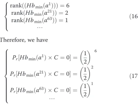
According to Equation 15, Hypothesis 1 is true only if all the Hbmin(αi), where 1≤ i≤ 2m−1, have the same rank. Unfortunately, this condition cannot always be met. For example, we have the following results over GF(26):
Therefore, we can get the conclusion that Hypothesis 1 proposed in [16-18] is not correct.
Figure 3 shows the probabilities that the elements in GF(26) are the roots of a random block with length l = 63 by simulations.
4. Blind recognition algorithm in soft-decision situations
4.1 Code length estimation and blind block synchronization
Soft outputs of the channel could provide more informa-tion about the reliability of each decision symbol. In this section, we propose an approach to improve the recog-nition performance by employing the soft decisions.
We define cr(x) to be the codeword polynomial of a
code block Cr. According to the algebraic principles of
cyclic codes, ifαiis a root ofcr(x), we havecr(αi) = 0 and Hmin(αi) × Cr = 0. In soft-decision situations, instead of
verifying whetherαiis a root of each block, we can cal-culatepj,i, the probability thatαiis a root of thejth block
in the received sequence as shown in Figure 2, and cal-culatepiin Equation 4 as follows:
pi¼
whereMis the number of blocks, as shown in Figure 2. The elements in an extension field GF(2m) can be sep-arated to some groups according to the minimal ele-ments over GF(2m). Each minimal polynomial has several roots in GF(2m), we call the set of them as a con-jugate element group in this paper. And the generator polynomial of a cyclic code can be factorized by some minimal polynomials as follows:
g xð Þ ¼m1ð Þx m2ð Þx …mpð Þx ð19Þ
Because the generator polynomial g(x) is a factor of a valid codeword polynomial c(x), the minimal polyno-mials in Equation 19 are also the factors ofc(x). So if an elementαi(1≤i≤2m−1) in GF(2m) is a root ofc(x), the elements which have the same minimal polynomial with αi
are also the roots ofc(x). Therefore, we can just calcu-late p′ λ(1 ≤ λ ≤ q), the probability that the minimal polynomial mλ(x)(1≤λ ≤q) is a factor ofcr(x), whereq
denotes the number of minimal polynomials over GF (2m). According to this idea, we can modify Equation 18 to Equation 20 to calculate p′ λ rather than pi. This
modification can reduce the calculation complexity be-cause the number of minimal polynomials over GF(2m) is severely lower than the number of elements in GF (2m). In Equation 20, p′ j,λ denotes the probability that
mλ(x) is a factor of the codeword polynomial of the jth block in the observed window as shown in Figure 2.
p′λ¼
And the IDEF defined in Equation 3 should be modi-fied to Equation 21:
ΔH¼−X
probability that a minimal polynomialmλ(x) is a factor of
matrixHbmin(mλ(x)) corresponding tomλ(x) and calculate the probability ofHbmin(mλ(x)) ×Cr= 0.
The coefficients of mλ(x) are in GF(2) and mλ(x) can be written as follows:
mλð Þ ¼x gexeþge−1xe−1þ⋯þg1xþg0 ð22Þ
whereeis the degree ofmλ(x).ge,ge−1,⋯,g1andg0are all in GF(2). According to these coefficients ofmλ(x), we can obtain the minimal polynomial-based binary, min-imal parity-check matrix Hbmin(mλ(x)) with the follow-ing steps.
1) We assume the code length island initialize a matrix Gas follows:
In Equation23, the number of rows and columns arel-eandl, respectively.
G¼
ge ge−1 … g1 g0 0 ⋯
0 ge ge−1 ⋯ g1 g0 0 ⋯
⋱ ⋱ ⋱ ⋱ ⋱ ⋱ ⋱
⋯ 0 ge ge−1 ⋯ g1 g0 0
B B @
1 C C A
ð23Þ
2) Transform the left e × e area of G to an identity matrixIby elementary row transformation as follows:
whereQis a matrix, which hasl-erows ande columns.
G¼ðI Qj Þ; ð24Þ
3) The minimal parity-check matrix can be obtained as follows:
Hbminðmλð ÞxÞ ¼ QTjIÞ
ð25Þ
According to the algebraic principles of coding theor-ies, we can calculate the syndromes corresponding to
Hbmin(mλ(x)) by Equation 25 [23]:
S¼½Sð Þ1 ;Sð Þ2 ;⋯;S nð Þr T
¼Hbminðmλð Þx Þ Cr; ð26Þ
wherenr is the number of rows inHbmin(mλ(x)), i.e. the degree ofmλ(x). Ifmλ(x) is a factor ofcr(x) and no error
occurs during the transmission, all syndromes should equal to zero. If the block contains errors ormλ(x) is not a factor of cr(x), not all the syndromes equal to zero. So
when the minimal polynomials, which are the factors of the generator polynomial, are correctly estimated, the probability of S= 0 is larger than the case of incorrect estimation of the minimal polynomials. p′ j,λ in Equa-tion 20 can be calculated as follows:
p′j;λ¼ 1 nr
Xnr
k¼1
Pr½SHð Þ ¼k 0;1≤k≤nr; ð27Þ
wherePr[SH(k) = 0][1≤k≤nr] is the probability ofSH(k) =
0(1≤k≤nr),kdenotes the corresponding row number of Hbmin(mλ(x)). In fact,p′j,λcalculated in Equation 27 is not
the probability thatmλ(x) is a factor of the codeword poly-nomial, it is just the mean value of the probabilities that the syndromes equal to zero. The true probability should be obtained by calculating the probability that all syn-dromes equal to zero. But as shown in section 3.2, the probability that all syndromes equal to zero is determined by the degree of the corresponding minimal polynomial for incorrect coding parameter estimations, the probability distribution is not uniform. But we use the mean value of
Pr[SH(k) = 0] to indirectly depict the probability that a
minimal polynomial is a factor of the codeword polyno-mial, the influence of the degree of the difference minimal polynomials is low. In this case, we can assume that for a
0 10 20 30 40 50 60
0 0.1 0.2 0.3 0.4 0.5
i
Probability of
i is a root
α
random data, the distribution of the probabilities of the minimal polynomials being factors of the codeword polynomials is approximately uniform.
Jing proposed the Adaptive Belief Propagation (ABP) method on soft-Input Soft-Output decoding of RS codes [26]. The main idea is adapting the parity-check matrix of the codes to the reliability of the received information bits at each iteration step of the iterative decoding procedure. This idea is also employed in [22] to achieve blind frame synchronization of RS codes. The adaptation procedure reduces the impact of most unreliable decision bits on the calculation of syndromes. In our work, we also utilize the adaptation algorithm introduced in [23] and [26] before using Equation 27. The adaptive processing for a given re-ceived codeword Cr and a binary minimal parity-check
matrixHbmin(mλ(x)) includes the following steps:
1) CombineHbmin(mλ(x)) andCrTto form a matrix H*
(mλ(x)) as follows:
(28)
wherer1,r2,…,r3are the soft-decision bits of the
codewordCr, {hk,u|1≤k≤nr, 1≤u≤l} are the
elements ofHbmin(mλ(x)) in GF(2).
2) Replace each ru (1 ≤ u ≤ l) in H*(mλ(x)) with their
absolute values to form a new matrixHrðmλð Þx Þ, adjust the positions of the columns inHrðmλð ÞxÞto make the first row inHrðmλð ÞxÞis ranked from the lowest to the highest and record the indexes. The absolute values of {ru|1≤u≤l} denote the reliabilities
of the received soft-decision bits. As shown in Equation29,j jri1≤j jri2≤⋯≤j jril andi1,i2,⋯,ilare the
column indexes ofri1;ri2;⋯;ril inH*(mλ(x)).
(29)
3) Transform Hrðmλð Þx Þ by elementary row operations to make the lastnrelements of the first column in Hrðmλð ÞxÞhas only one“1”at the top, as shown in
Equation30. The first row does not join the elementary transformations.
(30)
This transformation limits the influences of the most unreliable decision bit to only one syndrome element. Furthermore, we continue the elementary transform-ation on Hrðmið Þx Þ to limit the numbers of “1” in the followingnr–1 columns to one (except the first row), as
shown in Equation 31.
Hrðmλð ÞxÞ ¼
ri1
j j j jri2 j jri3 ⋯ rinr rinrþ1 ⋯ jril−1j j jril 1 0 0 ⋯ 0 x ⋯ x x 0 1 0 ⋯ 0 x ⋯ x x 0 0 1 ⋯ 0 x ⋯ x x
⋮ ⋮ ⋮ ⋱ ⋮ ⋮ ⋱ x x
0 0 0 0 1 x ⋯ x x 2
6 6 6 6 6 6 4
3 7 7 7 7 7 7 5
ð31Þ
When the left bottomnr×nr area becomes an indent
matrix, stop the operation. Then the last nr rows in Hr*(mλ(x)) form a new matrix. We recover its original
column orders and call it Hbmin_a(mλ(x)). Because the
transformation is elementary, the relationship Hbmin_a
(mλ(x)) × Cr = 0 in the hard decision situations still
exists if Cr is a valid codeword. So we can calculate
the probability Pr[SH(k) = 0] according to Hbmin_a
(mλ(x)). This replacement reduces the influences of the nr most unreliable decision bits.
In this paper, we assume that the transmitter is send-ing a binary sequence of codewords and ussend-ing a binary phase shift keying (BPSK) modulation, i.e. let +1 and−1 be the modulated symbols of 0 and 1. The modulation operation from code bit c to modulated symbols could be written as s= 1–2c, and we assume that the propa-gation channel is a binary symmetry channel which is corrupted by an additive white Gaussian noise (AWGN). For each configuration, the information symbols in the codes are randomly chosen. A received symbol r could be expressed asr=s+w, wherewis the AWGN.
Prðs¼ þ1Þ ¼Prðs¼−1Þ ¼1=2 ð32Þ
The noise w follows a normal distribution with the probability density function (PDF)
f xð Þ ¼ ffiffiffiffiffiffi1
So the conditional PDF ofris
f r sÞ ¼ ffiffiffiffiffiffi1
For a given received bitr, we can obtain the following conditional probabilities: vector corresponding to the random modulated vectors= [s1,s2,…,sn,sn+ 1,…]. We now calculate the conditional
Similarly, we can calculate the conditional probabilities ofs1⊕s2⊕s3= + 1 ands1⊕s2⊕s3=−1 as follow:
We define the XOR-SUM operation as X n
u¼1
⊗su¼s1⊕
s2⊕⋯⊕sn and assume that the conditional probabilities of XOR-SUM can be expressed as Equation 41:
Pr
According to the induction principle, the expression of the conditional probabilities in Equation 41 turns out to be true, and could be simplified as follows:
By employing Equation 44, we can calculate the
prob-adapted minimal binary parity-check matrix Hbmin_a (mλ(x)), uv represents the position of the vth non-zero
element in thekth row ofHbmin_a(mλ(x)).suv and ruv are the uvth modulated symbol on the transmitter and the
corresponding soft-decision output on the receiver, respectively.
In shortened code cases, a codeword with block length
l and shortened length ls can be obtained by choosing
the lastlelements from a codeword which has a regular length (l+ls) as follows:
where the firstlselements ofCware zeros. Therefore, we
can simply obtain the minimal parity-check matrices of the shortened codes by deleting the first ls columns of Hbmin(mλ(x)).
4.2 Recognition of generator polynomials
After the code length and synchronization position esti-mation, the extension field degree m corresponding to the being recognized code can also be obtained. Then we can list the minimal polynomials over GF(2m) and find out which ones are factors of the generator polyno-mial. These minimal polynomials can also be recognized according to the probabilities of syndromes equaling to zero.
In the procedure of the code length and synchronization position estimation, we have calculated the probability that a minimal polynomial is a factor of the received codeword polynomials. We assume that the estimated code length and extension field degree are landm, the number of minimal polynomials over GF(2m) is q and
m1(x), m2(x), …, mq(x) are the minimal polynomials
over GF(2m).
According to Equation 45, we can calculate the kth syndrome for a given minimal parity-check matrix of
Hbmin(mλ(x)). Equation 47 is the log-likelihood ratios
And we propose to calculate a likelihood criterion (LC) of mλ(x)(1 ≤ i≤ q) being a factor of the generator check matrix corresponding to the minimal polynomial
mλ(x),Mis the number of packets in the observed window
Was shown in Figure 2, nr is the number of the rows in Hbmin_a(mλ(x)), Lj SHbmin−aðmλð ÞxÞð Þk
is the LLR defined by Equation 47 and calculated at thejth block of the observed windowW. According to Equation 48, we can calculate the LCs of all the minimal polynomials over GF(2m). By com-paring the LCs, we can choose the minimal polynomials, LCs of which are obviously higher than others, as the estimated factors of the generator polynomial, then the generator polynomial is obtained.
However, we can test whether the product of several most likely minimal polynomials is a factor of the gener-ator polynomial to increase the successful recognition rate, because according to the adaptive processing of the parity-check matrices, the more parity equations we con-sider, the more we are able to construct a parity matrix which is parsed on less reliable bits. For the convenience of automatic recognition using computer programs, we propose the procedure including the following steps to estimate the optimal parity-check matrix:
Step 1: Calculate the LCs to form a vectorL:
L¼L mð 1ð Þx Þ;L mð 2ð Þx Þ;⋯;L m qð Þx ð49Þ
Step 2: Rank the vectorLfrom the highest to the lowest, in order to form a new vectorLRas follows:
LR¼ L mð λ1ð Þx Þ;L mð λ2ð Þx Þ;⋯;L mλqð Þx
ð50Þ
and record the indexes:
I¼λ1;λ2;⋯;λq ð51Þ
Step 3: Letωincrease from 1 toq, combine the binary minimal parity matrices for the minimal polynomials
mλ1ð Þx …mλωð Þx , in order to formHωas follows:
After adaptive processing forHω, calculate the LCs of
Hω×Cr= 0(1≤ω≤q) by Equation53and obtain the
Step 4: Find the maximal element ofLH, record the
corresponding matrixHω^
Step 5: According to Equations49and50, we can find the polynomialsmλ1ð Þx … mλω^ð Þx and write the generator polynomial as follows:
g xð Þ ¼mλ1ð Þx mλ2ð Þx …mλω^ð Þx ð55Þ
But in our work, we find that some minimal
polynomials are easily lost. These minimal polynomials have the minimal parity-check matrices with low rows, so the adaptive processing can only reduce the
influence for low number of unreliable decision bits. For example, consider the following minimal
polynomials corresponding to the elementsα1,α9and α0
respectively. Therefore, the number of rows of the binary minimal parity-check matricesHbmin(m1(x)), Hbmin(m2(x)) andHbmin(m3(x)) corresponding tom1(x), m2(x) andm3(x) are also 6, 3, and 1, respectively. So Hbmin(m1(x)),Hbmin(m2(x)) andHbmin(m3(x)) can limit
the influences of 6, 3, 1 unreliable decision bits after adaptive processing, respectively. Form2(x) andm3(x),
the LCs ofHbmin_a(m2(x)) andHbmin_a(m3(x)),
especiallyHbmin_a(m2(x)), may lower than the incorrect
minimal polynomials when the signal-to-noise ratio (SNR) is low. In this case, the ranking of LCs in Equation50may not be correct, so the generator polynomial recognition is failed. To solve this problem, we can additionally combine these minimal parity-check matrices withHω^ obtained in Step 4 described previously and check whether the corresponding
minimal polynomials are also factors of the generator polynomials. The details of the additional steps are listed below:
Step 6: List the binary minimal parity-check matrices over GF(2m) which have low rows:Hbmin(mL1(x)),Hbmin
(mL2(x)),…,Hbmin(mLη(x)), hereηrepresents the number
of binary minimal parity-check matrices with low rows. Step 7 Record LCmax¼LCðHω^Þand initialize a
Step 11: Output the newly obtainedHω^ as the final estimation of the parity-check matrix and get the generator polynomials according to the minimal polynomials corresponding toHω^.
5. General recognition procedure
In this section, we present the general procedure for the blind recognition of binary cyclic codes based on the princi-ples proposed in the previous sections. Before the recogni-tion, some prior information could help to estimate the possible range of the code length l. Then, we traverse all the possible values of code lengthland codeword starting positiontand choose the parameter pair (l,t) which maxi-mizes the IDEF defined in Equation 21 to be the estimated code length and block synchronization position. Note that to get the minimal polynomials for each code lengthlover an extension field GF(2m), we must know the field expo-nentmof the code. For an ordinary binary cyclic code, its code length is 2m−1, while the code lengthlof a shortened code is ¼22m
−1−ls, where ls is the shortened length.
Therefore, the minimal value of the field exponentmfor a code lengthlis the smallest integerksuch that<22k
. The maximal value of mshould be estimated with some prior information. For each code length l and synchronization position t, we traverse all the possible extension field degrees to calculate ΔH, and choose the maximum one as ΔH(l,t). After the code length estimation, we search for the minimal polynomials which are the factors of the generator polynomial by the algorithm described in section 4.2.
The general recognition procedure is listed below:
Step 1: According to some prior information, set the searching range of the code lengthl, i.e. set the minimal and maximal code lengthlminandlmax.
Step 3: Full fill the windowWwith the received soft-decision bits.
Step 4: Set the code lengthl=lmin.
Step 5: Set the initial synchronization positiontat 0, which is the starting position ofW.
Step 6: Assume the code length island the
synchronization position istand calculateΔH. Note that the windowWhas more than one assumed codewords, we calculate theΔHon all the codewords and compute the mean of them asΔH(l,t).
Step 7: Ift<l, then lett=t+ 1 and go back to step 6; ift=l, then jump to step 8.
Step 8: Ifl<lmax, then letl=l+ 1 and go back to step
5; ifl=lmax, then jump to step 9.
Step 9: Compare all the calculatedΔH(l,t), select the maximum one and get the corresponding values ofl, tandmas the estimated code length, synchronization position and the degree of the GF of the recognized codes, respectively.
Step 10: Let the code length and synchronization position be the estimated parameterslandt, fetchM codewords from the observed windowW. And list the minimal polynomials over GF(2m), which arem1(x), m2(x),…,mq(x).
0 0.2 0.4 0.6 0.8 1
0 0.05 0.1 0.15 0.2 0.25
p
Probability of mean(
p'j,
)=
p
ramdom data coded data
λ
Figure 4Probability density distribution ofp′λfor the coded and random data.
0 2 4 6 8 10 12 14
0 0.02 0.04 0.06 0.08 0.1 0.12 0.14
p'λ
λ
Step 11: Calculate the LCs of the minimal polynomials over GF(2m) by Equations47and48for theMpackets inW, and get the LC vector as shown in Equation49. Step 12: Recognize the generator polynomial follow the steps described in section 4.2.
Finally, we need a detection threshold to reject random data. When the received data stream is not encoded by binary cyclic codes, it can be considered that the data is random for all the coding parameters. The recognizer should give a report to reject the estimated parameters when the parity-check matrix is not likely enough.
We define the mean value ofp′j,λfor all the blocks in the observed window as follows:
mean p′j;λ
¼ 1
M
XM
j¼1
p′j;λ; ð58Þ
wherep′j,λis calculated by Equation 27 according to the recognized parity-check matrix Hω^, Hin Equation 27 is the recognized parity-check matrix Hω^ and nr denotes
the number of rows ofHω^. As shown in Figure 4, the dis-tributions of mean (p′j,λ) for random data and coded data with correctly estimated coding parameters are separated.
0 2 4 6 8 10 12 14
0 0.01 0.02 0.03 0.04 0.05 0.06 0.07 0.08 0.09
p' λ
λ
Figure 6Values ofp′λunder incorrect parameters.
The distances between the two distributions are mainly determined by the noise level, the number of rows inHω^, and the number of code blocks in the observed window. Experimentally, we propose the threshold δ to be about 0.6, in order to decide whether the data stream is random or not. After the estimation of the coding parameters, we calculate mean (p′j,λ) for all complete code blocks in the
observed window. If mean (p′ j,λ) is smaller than δ, we
propose to reject the recognition result.
6. Simulations
In this section, we show the efficiency of our proposed blind recognition algorithm by simulations. In the simulations,
we assume that the searching range of the code length is 7 ~ 128 and the observed window contains
N = 3,000 consecutive soft-decision bits from the BPSK demodulator. Meanwhile, we assume the data stream is corrupted by an AWGN on the channel.
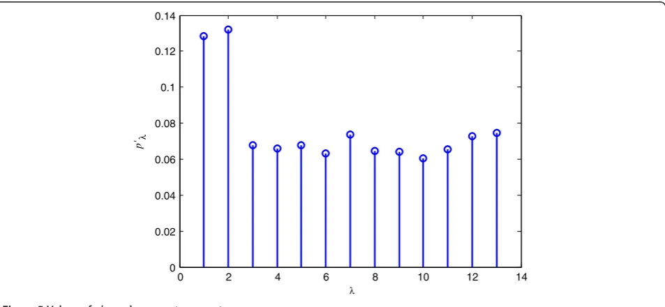
When employing the proposed algorithm to recognize the BCH (63, 51) code, the simulation results for code length and synchronization position recognitions are shown in Figures 5, 6, 7 and 8. The SNR isEs/N0= 5 dB
and corresponding BER is 10−2.19. Figure 5 shows the values of p′ λ defined in Equation 20 when l = 63 and
m = 6, and the block synchronization is achieved. Figure 6 is the case of another l and m. It is shown in
0 1 2 3 4 5 6
10-5
10-4
10-3
10-2
10-1
100
Es/N0(dB)
FRP
Hard BCH(63, 51)
Hard BCH(31,21)
Soft BCH(63, 51) Soft BCH(31,21)
Soft BCH(62,35)
Figure 8FRP of code length and synchronization position recognization on different SNRs for several binary cyclic codes.
0 2 4 6 8 10 12 14
-20 -10 0 10 20 30 40 50 60 70 80
L
(
m
(
x
))
λ
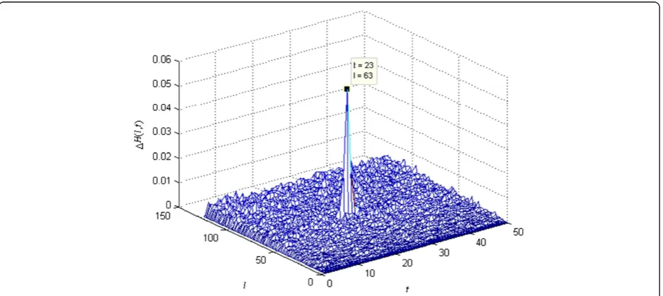
the two figures that when the code length and synchronization positions are correctly estimated, some minimal polynomials have higher probabilities to be factors of the received codeword polynomials. The obviously larger ones are calculated on the minimal polynomials which are factors of the generator polynomial. If the parameters are not correctly estimated, such feature will not exist. Figure 7 shows the IDEF ΔH for different code length l and synchronization positiont, while the first bit of the observed window is the 40th bit of a codeword. When l = 63 and
t= 23, the IDEF is the largest. Thus, we proposel = 63
and t¼23þlk kð ∈ZþÞ to be the estimation of the code length and synchronization positions, which are consistent with the simulation settings.
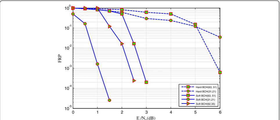
The performance of the algorithm is affected by the channel quality. In Figure 8, we draw the performance of the proposed algorithm when applied to code length recognitions of several different binary cyclic codes. The curves depict the false recognition probabilities (FRP) of the code length and synchronization position estimations on different SNRs. In Figure 8, we also compare the performance of our proposed recognition
0 2 4 6 8 10 12 14
-500 0 500 1000 1500 2000 2500 3000 3500 4000 4500
j
L
(
Hj
)
Figure 10Generator polynomial recognition of cyc (63, 36): sorted LCs.
0 1 2 3 4 5 6
10-8 10-6 10-4 10-2 100
Es/N0(dB)
FRP
Hard BCH(63, 51)
Hard BCH(63,39)
Hard BCH(30,20)
Soft BCH(63, 51)
Soft BCH(63,39)
Soft BCH(30,20) Soft cyc(63,36)
algorithm with the hard-decision-based RIDERS algo-rithm proposed in [16-18]. The PFR of our proposed al-gorithm fall rapidly when SNR increases, and it is much lower than that of the previous algorithms on each single SNR value.
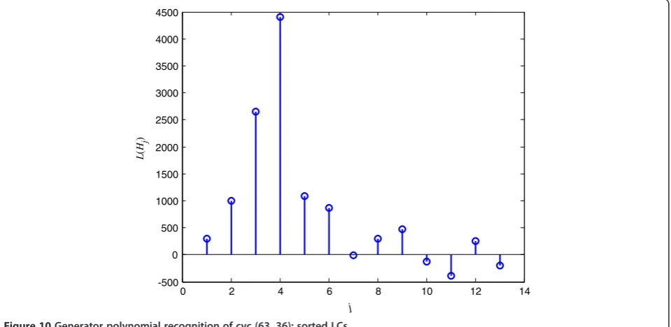
After the code length estimation, the generator poly-nomial could be recognized by searching for the min-imal polynomials which are factors of the generator polynomial according to the steps proposed in section 4.2. We assume that the data stream sent by the trans-mitter is coded by a cyclic code, the code length and in-formation length of which are 63 and 36, respectively. We call it cyc (63, 36) code in this paper. The generator polynomial of the code is the product of the following minimal polynomials, which includes low-degree min-imal polynomials:
The coded data is modulated by BPSK and corrupted by an AWGN with SNR Es/N0= 1.5 dB, and the correspond-ing hard-decision BER is about 4 × 10⁻². The recognizing procedure is shown in Figures 9, 10 and 11.
There are 13 minimal polynomials over GF(26), which are listed below:
Figure 9 shows the original LCs of different minimal polynomials over GF(26) to be factors of the codeword polynomials in the observed window. We rank the ori-ginal LCs from the highest to the lowest, in order to form a new vectorLRand record the indexI(defined in
Equation 51) as follows:
I¼½4 1 2 3 9 5 12 10 8 11 6 7 13
ð61Þ
Then we letωincrease from 1 to 13, combine the bin-ary minimal parity matrices for the minimal polynomials
mI(1)(x)…mI(ω)(x), in order to form Hω by Equation 52,
and calculate the LCs of Hω × Cr = 0(1 ≤ ω ≤ q) by
Equation 48. The LCs are shown in Figure 10. We can see that the LC of H4is the highest. H4 is obtained by combining the minimal parity-check matrices Hbmin(m4 (x)), Hbmin(m1(x)), Hbmin(m2(x)) and Hbmin(m3(x)). Fur-thermore, we list the low-degree minimal polynomials to check whether they are factors of the generator polyno-mial. The low-degree minimal polynomials are mL1(x) =
m5(x), mL2(x) = m9(x), mL3(x) = m11(x) and mL4(x) =
m13(x). We record LCmax= LC(H4) = 4,406.8 and execute the steps 8 ~ 10 described in section 4.2. Finally, we can ob-tain the values of LLR(H4,k)(1≤k≤4)) in Table 1.
It is obvious that LLR(H4,1) > 0.9 × LLR(H4) and LLR (H4,4) > 0.9 × LLR(H4,1). Therefore,H4,4 should be con-sidered as the finally recognized parity-check matrix. According to section 4.2, H4,4 is obtained by combining the minimal parity-check matrices Hbmin(m4(x)), Hbmin (m1(x)), Hbmin(m2(x)), Hbmin(m3(x)), Hbmin(m5(x)) and
Hbmin(m13(x)), so we can write the generator polynomial as follows:
g xð Þ ¼m1ð Þx m2ð Þx m3ð Þxm4ð Þx m5ð Þx m13ð Þx ð62Þ
The recognition result is accordant with the simula-tion settings.
Figure 11 shows the performance of the proposed gener-ator polynomial recognition algorithm when applied to several different binary cyclic codes. The curves show the
Table 1 LCs forH4andH4,k
Table 2 Error rejection rate
Es/N0(dB) ERP for BCH (63,51)
−1.0 1.00E0 4.06E-1 5.10E-1 <2E-6
−0.5 1.00E0 9.00E-3 4.51E-2
0.0 9.95E-1 6.67E-6 1.19E-4
0.5 9.90E-1 <2E-6 <2E-6
1.0 5.21E-1
1.5 1.32E-2
FRP on different noise levels. As Es/N0rises, the curves fall rapidly. We also compare our proposed algorithm with the previous hard-decision-based recognition algorithms pro-posed in [16-18]. It shows that the recognition performance is improved obviously in soft-decision situations.
After the coding parameter recognition, an additional testing program checks whether the data is random. The principle is described in section 4.2. We list the error-rejection-probabilities (ERPs) for some binary cyclic codes and the error-acceptance probabilities (EAP) for random data in Table 2. The ERP level is much lower than the FRP. Especially when the noise level is low enough, the ERPs are nearly zeros. And all the random data is rejected, that is to say, nearly no recognized result on random data is accepted.
7. Conclusion
A blind recognition method for binary cyclic codes for non-cooperative communications and ACM in soft-decision situations is proposed. The code length and synchronization positions are estimated by checking the minimal parity-check matrices. After that, the whole check matrix and generator polynomial are reconstructed by searching which minimal polynomials are factors of the generator polynomial. The recognition method proposed in this paper is based on an earlier published RIDERS al-gorithm with some significant improvements. By calculat-ing the probability that a minimal polynomial is a factor of the received codewords rather than checking whether an element in the extension field is a root of the codewords, we develop the RIDERS algorithm to soft-decision situa-tions. To calculate the probability that a minimal polyno-mial is a factor of a received codeword, we adopt some algorithms and ideas introduced in soft-decision-based decoding methods and blind-frame-synchronization approaches for RS and BCH codes in the literatures. Although we have always a loss of performance when these algorithms are applied in cyclic codes while they are particularly well suited for LDPC codes, the algorithm proposed in this paper still has a previously better recogni-tion performance for binary cyclic codes in a soft-decision situation than that in a hard-decision situation. And by the reliability-based adaptive processing, we reduce the influences of the most unreliability decision bits on the calculation of the syndromes, though the parity-check matrices of binary cyclic codes are not sparse. Moreover, the application field of the recognition method is extended to general binary cyclic codes in this paper, including shortened codes. To the best of our knowledge, this paper is the first publication in literature, which introduces an approach for complete-blind recognition of binary cyclic codes in soft-decision situations. Simulations show that our proposed blind recognition algorithm yields obviously better performance than that of the previous ones.
Competing interests
The authors declare that they have no competing interests.
Acknowledgements
This paper was supported by the graduate innovation fund of the National University of Defence Technology. And we wish to thank the anonymous reviewers who helped to improve the quality of the paper.
Received: 19 February 2013 Accepted: 20 August 2013 Published: 30 August 2013
References
1. V Choqueuse, M Marazin, L Collin, KC Yao, G Burel, Blind reconstruction of linear space-time block codes: a likelihood-based approach. IEEE. Trans. Signal. Proc.58(3), 1290–1299 (2010)
2. G Burel, R Gautier, Blind estimation of encoder and interleaver characteristics in a non cooperative context, inProceedings of IASTED International Conference on Communications, Internet and Information Technology(Scottsdale, AZ, 2003)
3. M Marazin, R Gautier, G Burel, Algebraic method for blind recovery of punctured convolutional encoders from an erroneous bitstream. IET. Signal. Proc.6(2), 122–131 (2012)
4. R Moosavi, EG Larsson, A fast scheme for blind identification of channel codes, inProceedings of the 54th GLOBECOM 2011(Houston, 2011) 5. AJ Goldsmith, SG Chua, Adaptive coded modulation for fading channels.
IEEE. Tran. Commun.46(5), 595–602 (1998)
6. M Marazin, R Gautier, G Burel, Dual code method for blind identification of convolutional encoder for cognitive radio receiver design, inProceedings of IEEE Globecom Workshops(Honolulu, 2009)
7. F Wang, Z Huang, Y Zhou, A method for blind recognition of convolution code based on Euclidean algorithm, inProceedings of IEEE WiCom
(Shanghai, 2007), pp. 21–25
8. J Dignel, J Hagenauer, Parameter estimation of a convolutional encoder from noisy observations, inProceedings of IEEE ISIT(Nice, 2007) 9. M Marazin, R Gautier, G Burel, Blind recovery of the second convolutional
encoder of a turbo-code when its systematic outputs are punctured. Mil. Tech. Acad. Rev.XIX(2), 213–232 (2009)
10. Z Yongguang, Blind recognition method for the turbo coding parameters. J. Xidian. Univ.38(2), 167–172 (2011)
11. M Marazin, R Gautier, G Burel, Blind recovery of k/n rate convolutional encoders in a noisy environment. EURASIP J. Wirel. Commun. Netw.
2011(168), 1–9 (2011)
12. M Cluzeau, Block code reconstruction using iterative decoding techniques, inProceedings of IEEE ISIT(Seattle, 2006)
13. J Barbier, G Sicot, S Houcke, Algebraic approach for the reconstruction of linear and convolutional error correcting codes, inProceedings of World academy of science, engineering and technology(Venice, Italy, 2006) 14. J Barbier, J Letessier, Forward error correcting codes characterization based
on rank properties, inProceedings of International Conferences on Wireless Communications(Nanjing, 2009)
15. Z Junjun, L Yanbin, Blind recognition of low code-rate binary linear block codes. Radio. Eng.39(1), 19–22 (2009)
16. W Niancheng, Y Xiaojing, Recognition methods of BCH codes. Elec. Warfare.
2010(6), 30–34 (2010)
17. Y Xiaojing, W Niancheng, Recognition method of BCH codes on roots information dispersion entropy and roots statistic. J. Detect. Contr.32(3), 69–73 (2010) 18. L Xizai, H Zhiping, S Shaojing, Fast recognition method of generator
polynomial of BCH codes. J. Xidian. Univ.38(6), 187–191 (2011)
19. S Lin, DJ Costello, Costello, Reliability-based soft-decision decoding algorithms for linear block codes, inError Control Coding: Fundamentals and Applications, 2nd edn. (Pearson Pretice Hall, Englewood Cliffs, NJ, 2004), pp. 395–452 20. R Imad, G Sicot, S Houcke, Blind frame synchronization for error correcting
codes having a sparse parity check matrix. IEEE. Trans. Comm.57(6), 1574–1577 (2009)
21. R Imad, S Houcke, Theoretical analysis of a MAP based blind frame synchronizer. IEEE. Trans. Wireless. Commun.8(11), 5472–5476 (2009) 22. R Imad, C Poulliat, S Houcke, G Gadat, Blind frame synchronization of
23. R Imad, S Houcke, C Jego, Blind frame synchronization of product codes based on the adaptation of the parity check matrix, inProceedings of IEEE ICC 2009(Dresden, Germany, 2009)
24. S Lin, DJ Costello, Linear block codes, inError Control Coding: Fundamentals and Applications, 2nd edn. (Pearson Pretice Hall, Englewood Cliffs, NJ, 2004), pp. 66–98
25. S Lin, DJ Costello, Introduction to algebra, inError Control Coding: Fundamentals and Applications, 2nd edn. (Pearson Pretice Hall, Englewood Cliffs, NJ, 2004), pp. 25–65
26. J Jiang, KR Narayanan, Iterative soft-input-soft-output decoding of Reed-Solomon codes by adapting the parity check matrix. IEEE. Trans. Infor. Theory.
52(8), 3746–3756 (2006)
doi:10.1186/1687-1499-2013-218
Cite this article as:Jinget al.:Blind recognition of binary cyclic codes. EURASIP Journal on Wireless Communications and Networking
20132013:218.
Submit your manuscript to a
journal and benefi t from:
7Convenient online submission 7Rigorous peer review
7Immediate publication on acceptance 7Open access: articles freely available online 7High visibility within the fi eld
7Retaining the copyright to your article