Stability and invariant manifold for a predator prey model with Allee effect

(1)

R E S E A R C H

Open Access

Stability and invariant manifold for a

predator-prey model with Allee effect

Ünal Ufuktepe

1*

_{, Sinan Kapçak}

1

_{and Olcay Akman}

2

*_{Correspondence:} unal.ufuktepe@ieu.edu.tr 1_{Department of Mathematics, ˙Izmir}

University of Economics, ˙Izmir, Turkey

Full list of author information is available at the end of the article

Abstract

Predator-prey models are similar to host-parasite and host-parasitoid models. We investigate the stability and invariant manifolds of a discrete predator-prey model by using center manifold theory which is not addressed in Çelik and Duman (Chaos Solitons Fractals 40:1956-1962, 2009), and Wanget al.(Ecol. Complex. 8:81-85, 2011).

1 Introduction

Predator-prey models are similar to host-parasite and host-parasitoid models. In this sys-tem, the predator does not live on the host. The prey serves as a food source for the preda-tor. There are many interactions between any pair of biological species; if two species compete for limited resources or one of the species preys upon the other, then one of the species is extinct.

The dynamic relationship between the interacting species has been one of the domi-nant themes in both ecology and mathematical ecology due to its universal importance. Recently many authors have explained the dynamics of competition and predator-prey models.

The following discrete time prey-predator system was studied by Çelik and Duman with an Allee eﬀect on the prey population [], and by Wang, Zhang, and Liu with Allee eﬀects both on prey and predator []:

Nt+=Nt+rNt( –Nt) –aNtPt,

Pt+=Pt+aPt(Nt–Pt),

()

where the parametersa,rare positive,Ntis prey density at timetandPtis predator density

at timet,ris the intrinsic growth rate. The termaNtisper capitapredator increase due to

prey consumption. Çelik and Duman [] claimed that the eigenvalues for the ﬁxed point (, ), which is a non-hyperbolic ﬁxed point, areλ=  andλ= , but the corresponding Jacobian matrix for this point is

J=

(2)

The Allee effect was first described by ecologist Allee []. The Allee effect may be caused by a variety of mechanisms applicable in small populations. The presence of Allee effects indicates that there is a minimal population size necessary for a population to maintain itself in nature. Interest in the dynamics of small populations, including Allee effects, has increased in recent years. Interest in how small populations interact with other popula-tions, including predator-prey systems, has also increased. Allee effects can occur at the higher tropic level (e.g., predator, parasite), at the lower level (e.g., prey, host), or during interaction between these levels. Adding Allee effects to a predator-prey system can be destabilizing, depending on the formulation of the equations and where Allee effects are added [].

In this paper, we consider the system subject to equations () when the predator pop-ulation is subject to an Allee effect which is more general than described by the system of equations (.) in [], and we also use the center manifold theory for non-hyperbolic equilibrium points []. with an Allee effect on the predator discussed by Wang, Zhang, and Liu []. The aim of this paper is to investigate stability of model () and analyze the stability of the exclusion fixed point, which is non-hyperbolic, for the particular cases whend=  andd=  by using the center manifold theory which is not addressed in [, ].

2 Stability of system (2)

In this section we investigate the stability condition for system ().

The ﬁxed points are (, ), (, ), and (_ar₊_r,_ar₊_r). The Jacobian matrix of the planar map

The Jacobian matrix for the extinction ﬁxed point (, ) is

J=

(, ) is unstable since one of the eigenvaluesJ is greater than . The Jacobian for the exclusion ﬁxed point (, ) is

J=

(3)

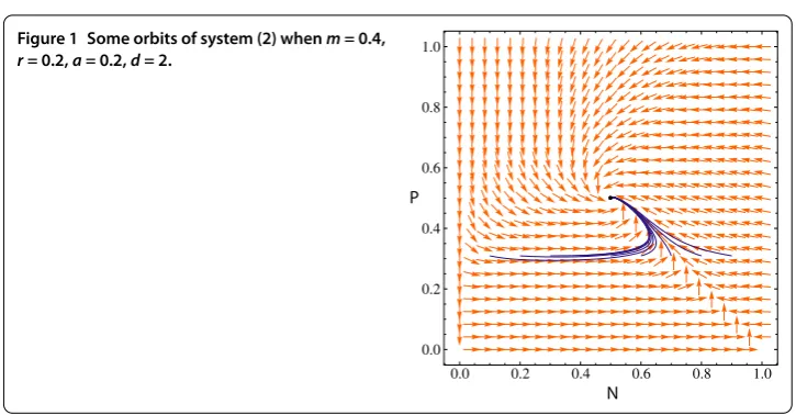
Figure 1 Some orbits of system (2) whenm= 0.4, r= 0.2,a= 0.2,d= 2.

We now discuss the coexistence of the ﬁxed point,i.e., (_a₊r_r,_ar₊_r): the Jacobian matrix for this point is

J∗= ⎛ ⎝ a+r–r



a+r –

ar a+r a(a+rr)+d

m+(_a₊r_r)d  –

a(ar+r)+d

m+(_ar₊_r)d

⎞ ⎠.

By using the Jury conditions [], after some manipulation, we obtain the following theo-rem.

Theorem  The positive ﬁxed point(_a₊r_r,_ar₊_r)is asymptotically stable if and only if

 <r(K+m)r+a(K–Kr) < a(K+m) –aKr– (K+m)(– +r)r,

where K= ( r a+r)

d_.

In Figure , we give the numerical evidence for some particular values of the parameters that the positive ﬁxed point is asymptotically stable.

3 Instability of an exclusion ﬁxed point

In this section, by using the center manifold theory, we show that for some values ofdfor system (), the ﬁxed point (, ) is unstable.

Theorem  For system(),the following statements hold true: (a) Ifd= ,then(, )is unstable.

(b) Ifd= ,then(, )is unstable.

Proof The eigenvalues of the Jacobian matrix corresponding to the system given in () at the point (, ) areλ=  –randλ= . Ifr> , then|λ|>  and (, ) is unstable.

Now, let us consider the case where  <r<  in which the eigenvaluesλ,λare subject to|λ|<  andλ= .

(4)

system is

According to system (), it becomes

ut+= ( –r)ut–avt+f˜(ut,vt),

Consider the center manifoldv=h(u). Let us assume that the maphtakes the form

h(u) = –r

au+αu

₊_β_u₊_O_u_, _α_,_β_∈_R_.

This leads to the evaluation of two constantsα andβ. The functionhmust satisfy the center manifold equation

h( –r)u–ah(u) +f˜u,h(u)–h(u) –g˜u,h(u)= .

By using the Taylor series expansion, we solve the functional equation above yielding

(5)

Thus, on the center manifoldv=h(u), we have the following map:

S(u) = –u(( +m)r

_u_{( +}_u_{) +}_ma_(–_m₊_ru_{( +}_u₎₎₎

m_a .

SinceS() =  andS() = –_mr< , the exclusion ﬁxed point (, ) is unstable. (b) Similarly, whend= , the new system is given by

ut+= (ut+ ) –r(ut+ )ut–a(ut+ )vt– ,

The Jacobian of the planar map which is given in () at the point (, ) is

˜

The equations in system () become

ut+= ( –r)ut–avt+f˜(ut,vt),

Consider again the center manifoldv=h(u). Let us assume that the functionhtakes the form

h(u) = –r

au+αu

₊_β_u₊_O_u_, _α_,_β_∈_R_.

Now we can evaluate the constantsαandβ. The functionhmust satisfy the center man-ifold equation

h( –r)u–ah(u) +f˜u,h(u)–h(u) –g˜u,h(u)= .

Utilizing the Taylor expansion, we solve the above functional equation

αr=  and

–aα+ (α+β)r+ r 

(6)

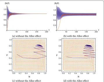
(a) without the Allee eﬀect (b) with the Allee eﬀect

(c) without the Allee eﬀect (d) with the Allee eﬀect

Figure 2 Trajectories of the prey-predator system: the Allee effect stabilizes the system.r= 2.5,a= 1.9, d= 2;(a),(c)m= 0;(b),(d)m= 0.1.

Solution of the above set of equations isα= ,β= –_mar. Hence

h(u) = –r

au– r

mau _.

Thus, on the center manifoldv=h(u), we have the following map:

R(u) =mau+r

_u_{( +}_u₎

ma .

Since R() =  andR() = , we need to calculate the Schwarzian derivative [] at the origin. Since the Schwarzian derivative at the origin is _mar > , we conclude that the ﬁxed

point (, ) is unstable.

(7)

(a) without the Allee eﬀect (b) with the Allee eﬀect

(c) without the Allee eﬀect (d) with the Allee eﬀect

Figure 3 Trajectories of the prey-predator system: the Allee effect destabilizes the system.r= 2.5, a= 0.5,d= 2;(a),(c)m= 0;(b),(d)m= 0.3.

Table 1 The Allee effect may stabilize or destabilize the system

Figure r a d m Fixed point Initial point

2(a), 2(c) 2.5 1.9 2 0 Unstable (0.3, 0.2) 2(b), 2(d) 2.5 1.9 2 0.1 Stable (0.3, 0.2) 3(a), 3(c) 2.5 0.5 2 0 Stable (0.3, 0.2) 3(b), 3(d) 2.5 0.5 2 0.3 Unstable (0.3, 0.2)

Competing interests

The authors declare that they have no competing interests.

Authors’ contributions

All authors contributed equally and signiﬁcantly in writing this paper. All authors read and approved the ﬁnal manuscript.

Author details

1_{Department of Mathematics, ˙Izmir University of Economics, ˙Izmir, Turkey.}2_{Department of Mathematics, Illinois State}

University, Normal, USA.

Received: 11 April 2013 Accepted: 7 November 2013 Published:03 Dec 2013

References

1. Çelik, C, Duman, O: Allee eﬀect in a discrete-time predator-prey system. Chaos Solitons Fractals40, 1956-1962 (2009) 2. Wang, W-X, Zhang, Y, Liu, C: Analysis of a discrete-time predator-prey system with Allee eﬀect. Ecol. Complex.8, 81-85

(2011)

3. Elaydi, S: Discrete Chaos: With Applications in Science and Engineering, 2nd edn. Chapman & Hall/CRC, London (2008)

4. Allee, WC: The Social Life of Animals. Book Club, London (1941)

(8)

10.1186/1687-1847-2013-348

Cite this article as:Ufuktepe et al.:Stability and invariant manifold for a predator-prey model with Allee effect.

References

1. Çelik, C, Duman, O: Allee effect in a discrete-time predator-prey system. Chaos Solitons Fractals40, 1956-1962 (2009) 2. Wang, W-X, Zhang, Y, Liu, C: Analysis of a discrete-time predator-prey system with Allee effect. Ecol. Complex.8, 81-85