Effect of scattering environment on estimation quality in V2I and V2V communications

(1)

R E S E A R C H

Open Access

Effect of scattering environment on estimation

quality in V2I and V2V communications

Elena Uchiteleva

*†

and Serguei Primak

†

Abstract

In this paper, we use a set of modulated discrete prolate spheroidal sequences (MDPSS) to represent a band-limited channel in the scenario with scattering from one or more clusters which can be used in both vehicle-to-infrastructure (V2I) or vehicle-to-vehicle (V2V) communication cases. Then we evaluate the performance of 2×1 space-time transmit diversity (STTD) system with Alamouti coding and imperfect channel estimation at the receiver. We consider examples of different scattering environments which represent vehicular communication in urban areas, derive expressions for autocorrelation function of channel gains and verify it by simulation. Scattering effect on estimation quality of the system is examined in terms of minimum mean square error (MMSE) and bit error rate (BER).

Keywords: Alamouti coding; MIMO channels; Scattering; Channel estimation; DPSS; Wiener filter; STBC; STTD

1 Introduction

High-quality channel state information (CSI) is essential for reliable performance of any practical communication system. The most popular approach is estimation via

training sequences (pilots) which are periodically inserted into the data stream [1-3]. The receiver extracts pilot sequences and, relying on the knowledge of channel statis-tics, performs the estimation. For simulation purposes, Rayleigh fading channels with Jake’s spectrum [4] and real-valued auto-covariance function are usually assumed, for example in works [1-3,5,6]. This is the worst case sce-nario, since there is no preferable angle of arrival (AoA). Therefore, it leads to unnecessarily large amount of pilots needed for reliable estimation, which is inefficient. More-over, practical channels usually exhibit non-symmetric spectrum and complex-valued auto-covariance functions. This work is focused on the estimation in a realistic urban environment. Hence, our goal is to account for a complex scenario, which describes scattering from one or more narrow clusters near the mobile, what results in the pres-ence of diffusive components in received signal coming from particular AoA, and to provide qualitative analy-sis of estimation in different real-life scattering scenarios.

*Correspondence: [email protected] †_{Equal contributors}

Department of Electrical and Computer Engineering, UWO, 1151 Richmond St., London, N6A 5B9, Canada

Measurements show, that realistic spectrum could be rep-resented as a sum of sub channels with a narrow and rectangular spectra [7,8]. Therefore, we can assume that the signal spectrum can be approximated as a group of distinct rectangles (corresponding to different clusters) and not as a classical Jake’s bathtub shape. Such repre-sentation allows us to perform more practical analysis of communication link and obtain more sensible results of estimation quality.

Channel basis expansion models (BEM) recently gained attention due to simplicity of their implementation [6]. For example, some models describing Jake’s spectrum include complex-exponential BEM [9] or polynomial BEM [10]. Discrete Karhunen-Loeve BEM is optimal in mean square error (MSE) sense [11,12]. In this expansion, optimal set of basis functions depends on the spectrum shape. It was shown in [11,13] that for a rectangular-shaped spectrum, a set of discrete prolate spheroidal sequences (DPSS) is opti-mal. Moreover, with the assumption that the spectrum can be approximated as an aggregate of rectangles, DPSS would provide a universal basis expansion. The channel model we use is described by a four-dimensional tensor of MDPSS representing channel response [14]. By mod-ulation of the bandwidth of a set of DPSS, we achieve different scattering scenarios with parameters defined by theoretical models or/and measurements [14].

(2)

Uchiteleva and PrimakEURASIP Journal on Wireless Communications and Networking2014,2014:129 Page 2 of 15 http://jwcn.eurasipjournals.com/content/2014/1/129

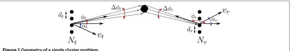
Figure 1Geometry of a single cluster problem.

V2V communication is accompanied by the move-ment of both receive and transmit sides with low ele-vation antennas and scatterers, which are assumed to be located on perimeters of multiple co-focal ellipses (with the receiver and the transmitter at ellipses’ foci). MDPSS channel model is a regular-shaped geometry-based stochastic model (RS-GBSM), which is very flexible in definition of the geometry and location of different clusters in Moderate Spatial Scale (MSS) or Small Spatial Scale (SSS) scenarios [15]. Furthermore, this model is suit-able for application in both V2I and V2V scenarios, as it gives us the control over definition of the motion of both communication sides. Thereafter, we evaluate how scat-tering from narrow clusters affects estimation quality of the mobile. These results could be further used in analy-sis and optimization of IP-level protocols, such as PMIPv6 [16].

Multiple-input single-output (MISO) is a very common scenario in the downlink of a cellular system. Therefore, in our work, we focused on a simple yet elegant cod-ing technique, the Alamouti scheme [4], which is used in some third/fourth generation wireless mobile standards. Pilot-assisted channel estimation is used with Wiener filter as a pilot filter [3]. In IEEE 802.11p, V2x commu-nication standard single-input single-output (SISO) sys-tems are postulated, but multiple-input multiple-output (MIMO) systems and their variations could be employed to improve the reliability of communications.

The remainder of our paper is organized as follows: in Section 2, the MDPSS-based channel model is reviewed and simulation results for one and two cluster case are presented. The 2×1 MISO communication system with Alamouti coding and channel estimation is described in Section 3. In Section 4, two different cases of environ-ment were tested and the performance of the system was evaluated via MMSE and BER. Moreover, an example of simulation of the channel at a real intersection was shown, followed by analysis of communication link. The conclusion is in Section 5.

2 Channel model

2.1 Geometry and channel response

In order to simulate a single cluster environment, we use a geometry shown in Figure 1: there are two horizontal

multi-element linear antenna arrays on both receiving and transmitting sides; the space between antennas contains a single scattering cluster. Impulse response H(τ,t) is assumed to be sampled at the rateFst(τ=n/Fst)and the channel is sounded at the rateFs(t=m/Fs). The carrier frequency isfc;Nr,Nt,dr,dtare the number of isotropic elements and the distance between them at receiving and transmitting antennas respectively;vrandvtare velocities at which receiver and transmitter move making anglesαt

Table 1 Example of simulation parameters for the channel with one scattering cluster

Param. Value Description

Nr 8 Number of antennas on the receiving side

Nt 8 Number of antennas on the transmitting side

vr 30 km/h Speed of the receiver

vt 0 km/h Speed of the transmitter

W 6 MHz Required channel half-bandwidth

fc 2 GHz Carrier frequency

dr,dt 0.5 Receive/transmit antenna spacing normalized to wave length

Pc 1 Power weights for clusters

φ0r 20° Azimuthal angle at which center of the cluster is seen to the receiver

φ0t 10° Azimuthal angle at which center of the cluster is seen to the transmitter

αr,_αt 0° The angle between broadside vector and movement direction φr 5° Angular spread seen from receiving side φt 8° Angular spread seen from transmitting side τ 0.3μs A mean delay associated with the cluster

τ 0.1μs Corresponding delay spread

Fst 50 MHz Sampling frequency in delay domain

Fs 250 Hz Rate of sampling in Doppler domain

irL 142 Length of the impulse response (num of samples)

L 1,024 Number of samples (in Doppler domain)

(3)

andαr with corresponding broadside vectors;φr andφt are azimuthal angles at which a cluster center is seen from receiving and transmitting sides, respectively. For simplic-ity, it is assumed that co-elevation anglesθt = θr = π₂ and there is no spread at this direction [14]. The cluster corresponds to time delayτ with delay spreadτ, as well as angle of departure (AoD) and angle of arrival (AoA)

φt,φrrespectively with angular spreadsφr,φtat each communication side. The Doppler shift is calculated as follows:

fD=

fc

c [vtcos(φt0−αt)+vrcos(φr0−αr)] , (1)

and the resulting Doppler spectrum widening is

fD=

fc

c [vtφt|sin(φt0−αt)| +vrφr|sin(φr0−αr)|] ,

(2)

A sample of the complete MIMO channel response takes a form of four-dimensional tensor [14]:

H4 = W4

nd are DPSS representing dimen-sions of a signal at the Receive, Transmit, Frequency and Doppler domains with ‘domain-dual domain’ prod-ucts:|φrNr_λdr cosφr0|,|φtN_λtdtcosφt0|,Wτ,Tmax₂fD respectively and Dr,t = 2φr,td_λr,tcosφ0r,t +1,Df =

2Wτ +1,D= fDTmax +1 the numbers of DPSS needed in each domain. ξnr,nt,nf,nd are Complex Gaus-sian i.i.d. variables with unit variance.W4is a tensor of modulating sinusoids described as follows:

W4=1w(r)×2w(t)×3w(ω)×4w(d), (4)

where is element-wise (Hadamard) product of two tensors and Tmax is the duration of the simulation. In

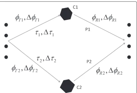
Figure 2Two-cluster environment example.

simulation of environment withNcclusters the total chan-nel response is a superposition of independently gener-ated normalized single-cluster responsesH4(k):

H4= total power. The auto-covariance functionRtot(τ)in this case is a sum ofNcauto-covariance functions of individ-ual one-cluster problems (due to linearity of the Fourier transform operation):

In this section, we present some results from simulation of a flat fading channel with one and two clusters and compare them to theoretical derivations, discussed pre-viously. An example of parameter summary of a single cluster from Figure 1 is given in Table 1, and parameters of a two-cluster case, which is depicted in Figure 2, are given in Table 2. If some parameters are not mentioned

Table 2 Two-cluster environment parameters

(4)

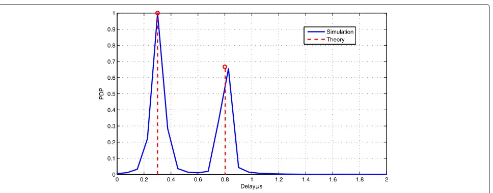
Figure 3PDP of one-cluster channel response,τ=0.3μs.

in the second table, they remain the same as in Table 1 and equal for both clusters. Simulation results for the one-cluster scenario are given in Figures 3, 4, and 5. Power delay profile (PDP) of this case is given in Figure 3, where there is a clear peak at delay associated with a particular clusterτ = 0.3μs with delay spread ofτ = 0.1μs. At Figure 4, we may see power spectral density (PSD) with resulting widened Doppler spectrum around frequency

fD ≈ 54.7 Hz with Doppler spread of fD = 4.8 Hz (calculated from Equations 1 and 2). The absolute value of auto-covariance function for this case,|R(τ)|, is given in Figure 5 as a function of normalized Doppler time

fD0τ, where fD0 = fc

|vt| + |vr|

c . In all figures, we can

see a good correspondence between the theory and the simulation.

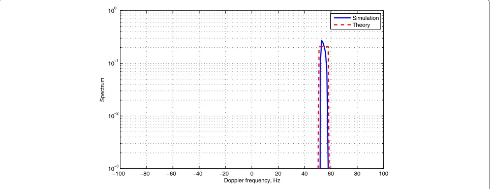
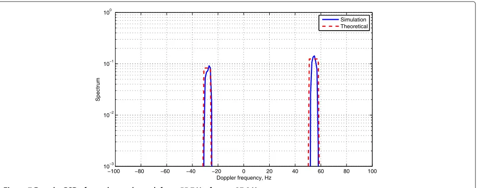
PDP and PSD of a two-cluster environment are shown in Figures 6 and 7, where we may observe a pick of received power at delaysτ1 = 0.3μs andτ2 = 0.8μs with power delay spread of 0.1 μs each (Figure 6) and widening of spectrum atfD1≈55 Hz and fD2≈ −28 Hz (Figure 7), the same frequencies that one may calculate from Equation 1. Theoretical and simulated envelopes of auto-covariance function are plotted in Figure 8. Again, there is a good agreement between simulation and theory.

3 Transmission system

We simulate the 2×1 MISO system with binary phase shift keying (BPSK) modulation and Alamouti coding scheme. Two transmitting antennas are assumed to be far enough from each other (the distance should be at least

(5)

Figure 5Envelope of the auto-covariance function of the channel process,|R(τ)|.

10 times greater than the carrier wavelength), so that each resolvable pass fades independently. For each symbol time the baseband equivalent model at the receiver is [4]:

y[m]=h1[m]x1[m]+h2[m]x2[m]+ξ[m] , (8)

wherehj[m] is a flat-fading Rayleigh channel gain between the transmitting antenna j(j = 1, 2) and the receiver, andξ[m] is the sampled additive white Gaussian noise,

ξ[m] ∼ CN(0,N0). In the Alamouti encoder [4], data stream is separated into two symbol blocks and sent from two antennas with rate of two bits per two symbol times. Two complex symbols u1 andu2 are transmitted in the following order:

(1) At first symbol time,x1[1]=u1,x2[1]=u2are

transmitted

(2) At second symbol time,x1[2]= −u∗₂,x2[2]=u∗₁are transmitted

(3) It is also assumed that the channel remains constant over two symbol times:h1[1]=h1[2]=h1,

h2[1]=h2[2]=h2(the quasi-static channel

assumption is valid when data rates are relatively high).

See Figure 9 for the visualization. Equation 8 could be rewritten in a matrix form [4]:

y[1] y[2]=h1 h2 u1 −u

∗

2

u2 u∗1

+ξ[1] ξ[2], (9)

(6)

Figure 7Doppler PSD of two-cluster channel,fD1≈55.7 Hz,fD2≈ −27.8 Hz.

or after some rearrangement,

y[1]

y[2]∗

=

h1 h2

h∗₂ −h∗₁ u1

u2

+

ξ[1]

ξ[2]∗

=Hu+ξ.

(10)

The columns of the square matrixHare orthogonal, hence one may separate Equation 10 into two orthogonal prob-lems. To decode informationyis projected onto each of the two columns of the matrix:h1h∗2

t

, [h2 −h∗1]t:

rj= ||h||uj+ξj, i=1, 2, (11)

whereh= [h1,h2]tandξj ∼ CN(0,N0)(ξ1,ξ2are inde-pendent), and then ML detection is performed for each of the decoded signals. The exact bit error probability for BPSK modulation was derived in [3] for a limiting case of perfect CSI and fully correlated channel gains,i.e. R(τ)=

1, at the receiver:

Pb= 1 4

2+

¯ γs

¯ γs+2

1−

¯ γs

¯ γs+2

2

, (12)

¯

γsis the average data signal-to-noise ratio (SNR) orEb/N0, when√Ebis the amplitude of the signal.

(7)

Figure 9Alamouti coding at time 1 (a) and time 2 (b).

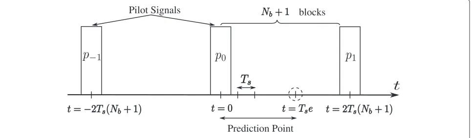
As the perfect CSI is not available in real-life com-munication, estimation of channel gains at the receiver is always required. We use pilot-assisted scheme with Wiener filter at the receiver [1,3,17]. The information codewords (or blocks of two symbol time lengths each) are divided into frames and interleaved with pilot sym-bols. Each frame containsNb +1 blocks: Nb blocks of information symbols and one block of pilot which is added at the beginning of the frame. The receiver pos-sesses the information about bit rate and the frame length. Therefore, it is able to extract pilot signals from the data stream and store them in the buffer of length 2M+1, where Mis an integer, which represents the number of pilots in the ‘future’ and ‘past’, i.e. the estimation and decoding processing is performed with delay ofMframe times. An example of a division into frames and pilot interleaving is visualized in Figure 10. Based on the infor-mation from the buffer and known channel statistics, the receiver performs channel estimation, decoding and

decision. In addition to the baseband representation (8), we express the pilot signal rp (which has energy 1, or 1/2 per antenna) and the bufferrp for each antenna as follows [3]:

rpj[m] = 1

√

2hj[m]+ξj[m] ,

rpj[m] =

rpj[m−M]· · ·rpj[m]· · ·rpj[m+M]

T . (13)

Due to channel variations in time, the filter coefficients should be recalculated every symbol slot within the frame, therefore they take the following form [3]:

he= 1

√

2

D0 2 + ¯γ

−1 p I2M+1

−1

ρe. (14)

Dedenotes a square matrix of size(2M+1)with entries given by:

(8)

Figure 11Estimation quality as a function of SNR and number of pilot signalsM.

De(k,l) = R(−eTs+(k−l)TsNb),

k,l = 1,. . ., 2M+1; e=0,. . ., 2Nb+1. (15)

I2M+1is identity matrix of size (2M+1), γ¯p denotes the average pilot SNR or pilotEp/N0,R(·)is channel auto-covariance function andρ_eis the(M+1)thcolumn ofDe. Thus, the matrixD0is a correlation matrix between pilot signals given in the buffer, andρ_eis a vector of correlations between the frame element at placeeand the nearest pilot signals. In a case of a static channelDe=D0andρe=ρ0 for anye. Estimated channel gains for antenna 1 and 2 are given by:

ˆ

h1[m,e]=hH_er1_p[m] , hˆ2[m,e]=hH_er2_p[m] . (16)

Indexmruns on frame slots with interval 2(Nb+1)Ts. It is worth mentioning that since we deal with Gaussian

distributed channel gains, Wiener filter is an optimal estimation filter.

BER of this scheme has been derived in [3] and is a func-tion of SNR and correlafunc-tion between the pilots ate=0 as the best-case scenario:

Pe=0= 1

4(2+ϒ) (1−ϒ)

2_. ₍₁₇₎

Here

ϒ =

4 1+ ¯γ_s−1

0 −

1

0

2−12

, (18)

and

0 =ρH0

D0

2 + ¯γp−1I2M+1

−1 ρ0,

1 =ρH₁

D0

2 + ¯γp−1I2M+1

−1

ρ0. (19)

(9)

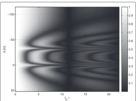
Figure 13Absolute value of autocorrelation function of channel gains,|Rd,fD0τ

|, V2I scenario.

In case of perfect CSI,R(τ)=1; therefore, (17) reduces to (12). Theoretical MMSE is given by

σ2

4 Simulation results of system performance in

different scenarios

In this section, we present some numerical results which evaluate the behaviour of the transmission system, dis-cussed in the previous section, in terms of estimation MMSE and BER, and analyze the influence of realistic scattering on the estimation quality. Thus, for example, Figure 11 shows estimation error for different number of pilots M in a one-cluster environment. The simulation was performed for the rate of 50 Kbps,Nb = 5,e = 0 and cluster parameters given in Table 1. As we would expect, the greater number of pilots reduces estimation

error for any SNR. It happens because the larger number of pilots provides more information to the receiver about correlation of channel gains; therefore, better estimation is achieved. There is a good convergence between theory and simulation.

Assuming that the exact geometry description of clus-ters and obstacles is available through different accessible applications like Google Maps© for 3D street view or through different global navigation and positioning satel-lite systems like GPS, GLONASS or QZSS, it is possible to model the geometry of any site of interest. Further, we present different scenarios of V2I and V2V cases.

4.1 V2I communication scenario

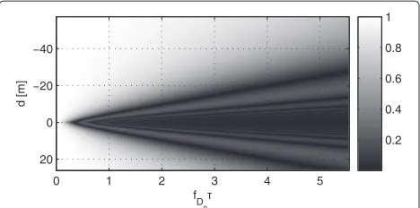
V2I example is shown in Figure 12. At this scenario, we assume that a mobile, for example a car, is moving along the road and passing under a big road sign. The base sta-tion is assumed to be far away. In this case, the angular spread φr changes as a function of time (or distance to the cluster) and, as we may see from the figureφr, increases as the car approaches the cluster. The expression for the varying angular spread is then:

φr(t)=2 tan−1 Table 1. Figure 13 shows behaviour of absolute value of auto-covariance function of channel gains as a function of Doppler time and a distance to the cluster. Negative dis-tance implies that the mobile is located on the left side of

(10)

Figure 15BER as a function of distance to the cluster.At SNR=10 dB, 50 Kbps rate and three pilot-based estimation, V2I scenario.

the cluster (according to Figure 12) and positive distance implies that it is located to the right. Cluster is located at

d = 0 m. It can be seen, that, as the mobile gets closer to the cluster, auto-covariance function decays faster. As a consequence, the pilot signals become less correlated, which results into higher estimation error. The behaviour of channel gains estimation MMSE as a function of dis-tance to the cluster at SNR = 10 dB and 50 Kbps rate with M = 1 and e = 0 for the estimation is shown in Figure 14 and the resulting BER is given in Figure 15. If we compare BER curves to Perfect CSI case (or error-free estimation), we may see the initial increase of 4 dB in BER, which happens because of the estimation based on three pilots only. It can be improved with use of more pilots (up to 10). Further increase in BER is introduced as the car nears the cluster. We may observe, that the effect of clus-ter’s presence is more pronounced at longer frames. If the

frame is built of more than 100 blocks, MMSE increases dramatically when the vehicle approaches the cluster. For example, for 200 block frames, the increase in MMSE is more than 10 times with resultant increase in BER by 4.7 dB (see Figure 15), when the car is under the road sign. Therefore, this kind of clusters produce significant shadowing effect on communication session. On the other hand, this apparent decrease of communication quality is fleeting and does not last more than a couple of seconds (in a current setting).

4.2 V2V communications scenario

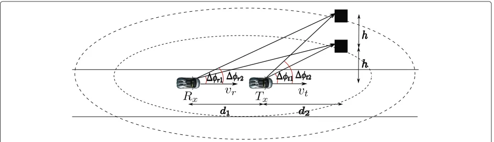
The example of V2V scenario is shown in Figure 16. Now, the receiver and the transmitter are moving at the same direction and are passing two identical clusters, which are located on the side of the road. For simplicity,

(11)

Figure 17Absolute value of auto-covariance function of channel gains,|Rd,fD0τ

|, V2V scenario.

we assume that both clusters are located on the same perpendicular to the mobile movement vector with equal distance between each other and the road,h=10 m. Fur-ther, we assume that the angular spread of both clusters is the same and approximately does not change as mobiles pass by,φ1,φ2≈ 5°. More complicated cases without identical clusters and varying angular spread are straight forward. The initial angles between the first cluster cen-tre and the vectors of movement of the receiver and the transmitter respectively areφr10 = 5°,φt10 = 7°. Hence,

the angle between mobile movement vectors and the cen-ter of the second cluscen-ter is calculated from: φr20,t20 =

tan−1 2 tan φr10,t10

and equals approximately 100and 140. Each one of anglesφr1(t),φr2(t),φt1(t),φt2(t)changes in accordance with distance change (as a function of time) between clusters and the car:

Figure 18Estimation MMSE as a function of distance to the cluster.With respect toRxand a frame lengthNbat SNR=10 db and three pilot-based estimation, V2V scenario.

φr,t,i(t)=tan−1

htan φr0,t0,i

h−vttan φr0,t0,i

, i=1, 2. (22)

The snapshot of auto-covariance function in the case when both vehicles’ speeds equal 30 km/h is shown in Figure 17. Resulting estimation MMSE and BER are shown in Figures 18 and 19. Figure 18 shows estimation error as a function of frame length Nb and the distance from the cluster with respect to the receiver. As we can see, longer frames increase MMSE due to decreasing corre-lation between pilots. On the graph we can distinguish two notches at d = −40 m and d = 0 m, where the system experiences quick decrease in estimation MMSE, corresponding to the vehicles’ location strictly perpen-dicular to clusters. This behaviour has a simple explana-tion: when one of the mobiles is located at the minimal distance to clusters, both clusters have equivalent angular parameters, what in terms of auto-covariance function equals to summation of two equally modulated sink func-tions; therefore, when absolute value is taken, it behaves like a one-cluster case: a slow decay in correlation as an absolute value of a pure sink function. Or effectively, the mobile ‘sees’ one cluster with unity power. The greatest estimation error is induced when vehicles are located at the different sides of the cluster (−40 m ≤ d ≤ 0 m on the graph). From the graph of BER (Figure 19), we see that (as in V2I case), there is an initial recession of 4 dB in performance because of estimation based on three pilot signals, and further increase of 3.8 dB is introduced because of the cluster presence. In this scenario, the effect of clusters is not fleeting as in the previous case (V2I scenario) and starts affecting the communication qual-ity, when the mobile is located as far as 80 m from the cluster.

(12)

Figure 20Real Street View, Wonderland Rd. and Oxford St. intersection, London, Ontario, Canada, ON N6H.

(13)

Figure 23The geometry of the site around the mobile.

4.3 Simulation of a real intersection in V2I case

In this section, we show how the channel model, discussed previously, can be used for simulation of a communica-tion link at the real-life site, located at the interseccommunica-tion of Wonderland Road and Oxford Street at London, Ontario, Canada, as shown in Figure 20 (East of Wonderland Road view to the North-West). In this example, we used Google Maps© application for measurements of distances and cluster dimensions due to its accessibility, but any other mapping and location application can be used for the sim-ilar analysis. Let us assume, that a mobile, equipped with the discussed communication system, is passing through the intersection with a speed of 30 km/h and moving to the North along Wonderland Road. Let us assume as well that there is a downlink between the mobile and a cellular tower located on the roof of one of the buildings on the left-hand side of the road, at the address 720 Wonderland Rd., which is approximately at the distance of 400 m to the North from the intersection, see Figure 21 (a view on the intersection at the Google Maps©). Analyzing the site, we may identify several clusters in the vicinity of the mobile: Petro-Canada and Esso gas stations on the Western side of Wonderland Road (and on opposite sides of Oxford), a big metal poster, a convenience store near the Esso gas station, and Malibu Restaurant West Inc. to the North from Esso, see Figure 22. All the rest of the buildings and obstacles are either shadowed by these four clusters (for example, cluster 5 at Figure 22) or too far to contribute to the signal

scattering with respect to the current mobile location (but might be taken into consideration when recalculating the communication site layout as the mobile moves forward and approaches them). The distances, angles and angular spreads of each cluster can be easily measured and cal-culated using Google Distance Measurement Tool©. The final cluster layout is shown in Figure 23, and parameters of each cluster are listed in Table 3. Powers of clusters were chosen arbitrary for simplicity purposes, but could be ver-ified through more elaborate calculations, for example with use of Radar Equation [18]. Auto-correlation func-tion of the channel in this scenario is shown in Figure 24 as a function of normalized Doppler time and distance to

Table 3 Parameters of clusters in scenario on Wonderland Road and Oxford Street intersection

Cluster 1 Cluster 2 Cluster 3 Cluster 4

φr(°) 121.3 46.1 26.3 22

φr(°) 25.7 35.7 2.4 16.7

φt(°) 134.8 143.9 134.3 134.9

φt(°) 3.4 5.1 0.6 6

τ(μs) 1.68 1.43 1.38 1.38

τ(μs) 0.09 0.08 0.003 0.01

h(m) 55.7 64.55 31.88 42.78

(14)

Figure 24Auto-correlation function in a real-life scenario, Oxford Street - Wonderland Road intersection, London, ON, Canada.

cluster 2. As it is seen from the graph, cluster 1 almost does not contribute to the fading, cluster 2 and cluster 4 make the major contribution, and we may distinguish them on the auto-covariance function graph. Contribu-tion of cluster 3 is merged with that of cluster 2, because this cluster is small and is located really close to the big cluster 2; therefore, the mobile is not able to differentiate between them. Effectively, it adds up to the power of clus-ter 2. Overall, the correlation snapshot appears blurred with a lot of grey levels corresponding to the correla-tion of 0.3 to 0.6 with no very pronounced dark areas (a very low correlation), as we saw in previous cases. The reason is that in this scenario, the distances between the mobile and clusters are bigger than in previous cases (30

to 64 m compared to 10 to 20 m) as well as angular spreads (25° to 35° compared to 10° to 19°). An exam-ple of MMSE and BER for 200 blocks frame-length and with three pilot signals prediction at 50 kbps is shown in Figure 25, where we can see the influence of clus-ters at 0 and around 40 m (with respect to the second cluster).

In a similar way, the communication in any type of ter-rain, containing multiple obstacles, can be analyzed. Of course, extension to more complicated scenarios describ-ing bigger number of clusters with non-symmetrical allo-cation is straightforward. Also, another various kinds of modulation and transmission schemes could be evaluated to improve the overall performance of the system.

(15)

5 Conclusion

In this paper, MDPSS-based channel model was adopted for representing a practical environment containing one or more clusters whose geometry is known and prede-fined. It mimics realistic channels with non-symmetric spectra and complex-valued auto-covariance function, what allowed us to obtain more reasonable results. STTD communication system with Alamouti coding and pilot-based channel estimation was described in detail and applied to two different realistic scenarios: one of them depicts V2I communication with a mobile moving under a big cluster located on the way of the mobile, like a road sign. The other one sketched V2V case with two similar clusters located on one side of the road and two communi-cating mobiles passing by. The analysis of estimation qual-ity were performed for each scenario. In both cases, an increase in estimation MMSE was detected in the vicinity of clusters resulting in the degradation of system perfor-mance in terms of BER. The effect of perforperfor-mance down-grading is larger in cases of longer frames between pilot signals, as a straightforward result from quickly decaying auto-covariance function of channel gains in occurrence of clusters in the environment. In the first scenario, the increase in MMSE and BER was higher than in the second scenario, although with shorter duration. Finally, an exam-ple of imexam-plementation of aforementioned channel model in simulation of communication at a real-life intersection was presented and discussed. It is worth mentioning that due to flexibility of the MDPSS simulator, the description of a vast variety of different scenarios is available, allowing one to easily test any kind of environment with different positioning of clusters in both V2V and V2I cases.

Competing interests

The authors declare that they have no competing interests.

Acknowledgements

The authors are supported by NSERC Canada.

Received: 30 January 2014 Accepted: 16 June 2014 Published: 11 August 2014

References

1. JK Cavers, An analysis of pilot symbol assisted modulation for rayleigh fading channels. IEEE Trans. Veh. Tech.40, 686–693 (1991)

2. K Almustafa, S Primak, T Willink, K Baddour, On Achievable Data Rates and Optimal Power Allocation in Fading Channels with Imperfect Channel State Information, inIEEE 4th International Symposium on Wireless Communication Systems(Trondheim, Norway, 17–19 Oct. 2007) 3. J Jootar, JR Zeidler, JG Proakis, Performance of Alamouti space-time code

in time-varying channels with noisy channel estimates, inIEEE Wireless Communications and Networking Conference(New Orleans, LA, USA, 13–17 March 2005)

4. D Tse, P Viswanath,Fundamentals of Wireless Communication(Cambridge University Press, New York, 2005)

5. H Zhu, B Xia, Z Tan, Performance analysis of Alamouti transmit diversity with QAM in imperfect channel estimation. IEEE J. Selected Areas Commun.29, 1242–1248 (2011)

6. Z Tang, RC Cannizzaro, G Leus, P Banelli, Pilot-assisted time-varying channel estimation for OFDM systems. IEEE Trans. Sygnal Process. 55, 2226–2238 (2007)

7. J Andersen, N Blaustaein,Multipath Phenomena in Cellular Networks

(Artech House, Norwood, 2002)

8. N Blaunstein, M Toeltsch, J Laurila, E Bonek, D Katz, P Vainikainen, N Tsouri, K Kalliola, H Laitinen, Signal power distribution in the Azimuth, elevation and time delay domains in urban environments for various elevations of base station antenna. IEEE Trans. Antenn. Propag.54, 2902–2916 (2006) 9. MK Tsatsanis, GB Giannakis, Modeling and equalization of rapidly fading

channels. Int. J. Adapt. Control Signal Process.10, 159–176 (1996) 10. DK Borah, BD Hart, Frequecy-selective fading channel estimation with a

polynomial time-varying channel model. IEEE Trans. Commn.47, 862–873 (1999)

11. H van Trees,Detection, Estimation and Modulation Theory: Part 1, 1st edn. (Wiley, New York, 2001)

12. M Visintin, Karhunen-Loeve expansion of fast Rayleigh fading process. IEEE Electron. Lett.32, 1712–1713 (1996)

13. T Zemen, C Mecklenbrauker, Time-variant channel estimation using discrete prolate spheroidal sequences. IEEE Trans. Signal Process. 53, 3597–3607 (2005)

14. SJ Haghighi, S Primak, V Kontorovich, E Sejdic, Wireless communications and multitaper analysis: applications to channel modeling and estimation, inMobile and Wireless Communications Physical Layer Development and Implementation(InTech Publishing, Rijeka, 2010) 15. C-X Wang, X Cheng, Vehicle-to-vehicle channel modeling and

measurements: recent advances and future challenges. IEEE Commun. Mag.47, 96–103 (2009)

16. J-H Lee, T Ernst, N Chilamkurti, Performance analysis of PMIPv6-based network mobility for intelligent transportation systems. IEEE Trans. Veh. Tech.61, 74–85 (2012)

17. S Haykin,Adaptive Filter Theory, 4th edn. (Prentice Hall, Upper Saddle River, 2001)

18. L Bernardo, A Roma, N Czink, A Paier, T Zemen, Cluster-based scatterer identification and characterization in vehicular channels, in11th European Wireless Conference - Sustainable Wireless Technologies (European Wireless)

(Vienna, Austria, 27–29 April 2011), pp. 1–6

doi:10.1186/1687-1499-2014-129

Cite this article as:Uchiteleva and Primak:Effect of scattering environment

on estimation quality in V2I and V2V communications.EURASIP Journal on

Wireless Communications and Networking20142014:129.