R E S E A R C H
Open Access
Stability analysis of a two-patch
predator–prey model with two dispersal
delays
Guowei Sun
1and Ali Mai
1**Correspondence:[email protected] 1Department of Mathematics and
Information Technology, Yuncheng University, Yuncheng, China
Abstract
This paper deals with a predator–prey model with both species in the
delayed-dispersal case in a two-patch environment. The purpose of this paper is to study the effect of two dispersal delays on the stability of three equilibria. It turns out that the stability of the trivial equilibrium and the boundary equilibrium is
delay-independent. However, the stability of the coexistence equilibrium is
delay-dependent. Numerical simulations are performed to demonstrate the obtained results.
MSC: 92B05; 34K20; 34K18; 34K10
Keywords: Dispersal; Delay; Stability; Bifurcation; Predator–prey model
1 Introduction
The relationship of predator and prey is prevalent in nature and hence is one of the most important themes in ecological and mathematical models. Since the Lotka–Volterra predator–prey model was formulated, various predator–prey models have been studied by incorporating additional ecological concepts into the classical Lotka–Volterra model, such as functional responses, dispersal and time delay. In predator–prey models, dispersal will represent migration of either the prey population, the predator population, or both [1,2].
Population dispersal is very common in ecology. Species migrate from one patch to an-other patch, due to some kinds of factor in the initial patch. For instance, a prey species will choose to move on the basis of resource availability and predation risk, while predators tend to migrate to the better patch to gain more prey. In nature, lack of food, competition, sex, age, lack of security (mainly for the prey), climatic conditions, season, overpopula-tion in a patch—these factors make species move from a patch to another [3]. For exam-ple, in aquatic environments, many zooplankton species exhibit vertical movements each day due to light and food. During the day time, some species migrate downwards into the darkness to reduce the predation risk by fish, while at night time, these species move upward to consume the phytoplankton [4]. There has been great interest in the study of mathematical models of populations with species dispersal among patches, such as a sin-gle population dispersal [5–8], and the dispersal of both prey and predator among patches [9–11].
It is worth pointing out that most of the research work in population models with patchy structures assumed the dispersal to be instantaneous. In fact, species movement between patches takes some time. Recently, Zhang et al. considered a predator–prey metapopula-tion model with travel time delay and showed that such delay can stabilize and destabilize the system [8].
To the best of our knowledge, there is little research on joining considerations of mi-gration and dispersal delay in biological models. It is challenging to add time delays to predator–prey models for the mathematical analysis. Delay may change the stability of dy-namics and Hopf bifurcation may occur. Motivated by the above predator–prey model, we will integrate dispersal of both species and dispersal delays into a two-patch Rosenzweig– MacArthur predator–prey model. We shall investigate how the dispersal and dispersal delays interact to affect the stability of the predator–prey metapopulation model.
The rest of the paper is organized as follows. The formulation of mathematical model is presented in Sect.2. The stability analysis of our model at three equilibria are given in Sect.3. Then numerical simulations based on the analysis are reported in Sect.4. Finally, we conclude the paper by a short discussion.
2 Model formulation
In this paper, our model assumes that the prey has a logistic growth rate and a predator has a Holling-type II functional response on each patch. The predator decays exponen-tially in the absence of prey. And we suppose that these patches are identical and the prey and predators can randomly move between two patches. During dispersal, migrating pop-ulations are assumed not to participate in the predator–prey interaction due to the two species being in different habitats. Thus, we propose a two-patch predator–prey model with dispersal of both species:
respectively.ris the prey growth rate.Kis the carrying capacity of prey.ais the maximum and constant rate of prey consumption per predator.bis the prey density where the attack rate is half-saturated.cis the inverse of yield.δis the predator mortality.DandMare the dispersal rate of prey and predators among patches, respectively.η1 andη2 are the dispersal time of prey and predators, respectively.
A series of change of variables is carried out to reduce the number of parameters:Hi=
bhi,Pi=bracpi,t=as,ηi=τai,κ=Kb,ε=ra,d=Da,m=Ma,μ=δa, and this yields the model
Theorem 2.1 Consider(2.2)with d= 0and m= 0,the following conclusions hold:
(2) The predator-extinction equilibrium(κ, 0)is stable whenμ>1+κκ. (3) The coexistence equilibrium(h∗,p∗)exists if and only if0 <μ<1+κκ. (4) The coexistence equilibrium is globally stable whenκκ–1+1<μ<1+κκ. (5) There is a unique globally stable limit cycle if0 <μ<κκ–1+1.
3 Stability analysis of the equilibria
Model (2.2) has three equilibria representing different outcomes of the ecological system:
E0= (0, 0, 0, 0) : extinction of both the prey and the predator in each patch;
Now we linearize system (2.2) at an equilibrium (h,p,h,p) and substitute an exponential solution, and we obtain the characteristic equationdetJ= 0 with
J= determines the local stability of equilibria. The equilibrium is stable if and only if all the characteristic roots have negative real part. In the following, we will analyze the stability of our model (2.2) at three equilibria, respectively.
3.1 The stability analysis ofE0
Inserting the trivial equilibriumE0 into the characteristic equationdetJ= 0, we get the characteristic equations
Based on the technique of [13–15], the stability change at the equilibrium can only hap-pen when characteristic roots appear on or cross the imaginary axis asτ increases. Here we assume thatε= 2d, then we look for a pair of purely imaginary roots of the character-istic equations (3.1).
Setλ=iωwithω> 0. By substitutingλinto the first equation of (3.1), then separating the real and imaginary parts, we get
⎧
Similarly, for the second equation of (3.1), there is a pair of purely imaginary roots±iω0 withω0=
d2– (ε–d)2.
For the third equation and the last equation of (3.1), by using the same method, we have ω2=m2– (μ+m)2< 0. Thus, there are no purely imaginary roots for the last two equations
of (3.1).
Lemma 3.1 Suppose at certainτ1,the first and second equation of characteristic equation
(3.1)have purely imaginary roots±iω.Then
dRe(λ)
Proof It follows from the first equation of (3.1) that
dλ
For the second equation of (3.1), the conclusion of the lemma also holds. The proof is
complete.
By Lemma3.1, we know thatdRedτ(λ)
1 |λ=iω0> 0. This indicates that, asτ1increases, for the first and second equation of (3.1), the characteristic roots cross the imaginary axis through
±iω0atτ =τ1from left to right and the number of characteristic roots with positive real parts is increased by 2.
3.2 The stability analysis ofE1
Using the same procedure as the stability analysis ofE0, inserting the equilibriumE1into the characteristic equationdetJ= 0, we get the characteristic equations
⎧
Substituting λ=iωwith ω> 0 into these characteristic equations (3.3), and separat-ing the real and imaginary parts, we can calculate that ifμ>1+κκ,|cosωτ1|= 1 + εd> 1,
|cosωτ2|= 1 –
κ
1+κ–μ
m > 1, which means there is no solutions of (3.3) can appear on the
imaginary axis for anyτi. Therefore,E1is locally asymptotically stable whenμ>1+κκ.
For case (2), if 0 <μ< κ
1+κ, by the expression ofcosωτ1, the first and second
equa-tions of (3.3) have no imaginary roots. However, the third and fourth equaequa-tions admit purely imaginary roots±iωwithω=
two equations have no imaginary roots while if 0 <μ< κ
1+κ – 2m. It is easy to show that
sign(d(dReτλ)
2 )|λ=iω=sign(ω
2) > 0, Note that equilibriumE
1is unstable withτ1=τ2= 0 in case (2). So when 0 <μ< κ
1+κ,E1remains unstable asτ1andτ2increase.
3.3 The stability analysis ofE2
In this subsection, we assume that 0 <μ<1+κκ to ensure the coexistence equilibriumE2 exists. InsertingE2into the characteristic equationdetJ= 0, we get
⎧
Whenτ1=τ2= 0, the characteristic equation becomes
⎧ ⎨ ⎩
λ2–Aλ+B= 0,
λ2– (A– 2d– 2m)λ– 2m(A– 2d) +B= 0.
Therefore, the coexistence equilibrium is stable ifA< 0, otherwise unstable.
Whenm= 0, this implies that prey disperses only. Based on the results of [8], we sum-marize the related conclusions in the following theorem.
Case (i) d∈(0,A/2):the coexistence equilibriumE2remains unstable forτ1> 0.
Case (ii) d∈(A/2,A):the coexistence equilibriumE2remains unstable forτ1> 0.
Case (iii) d∈(A,∞):there may exist stability switches.
When both species are mobile, due to the presence of two different time delays in char-acteristic equations, it is usually difficult to analyze the transcendental equation with two delays. Actually, finding all the characteristic roots of Eq. (3.4) have negative real parts is hopeless [16]. This indicates the difficulty in investigating the distribution of the zeros of Eq. (3.4). Thus, we mainly numerically examine how the two dispersal delays affect the stability of the coexistence equilibrium in our model in the next section.
4 Numerical simulations
From the above section, we know that the stability of the trivial equilibriumE0and the boundary equilibriumE1is relatively simple. However, the stability analysis of the coex-istence equilibriumE2is complicated. Therefore, in this section, we mainly present some numerical examples of our model (2.2) and investigate that the effect of delay on the sta-bility and instasta-bility of the coexistence equilibriumE2. Based on Theorem3.2, we display the numerical simulations in each case.
Example1 We take parameter valuesε= 1,κ= 2,μ= 0.4,d= 0.1,m= 0.05,τ1= 2,τ2= 2. This set of parameter values lead toA= –0.09 < 0. In this case,E2= (0.71, 1.10, 0.71, 1.10) is locally asymptotically stable. Due to the identical patch, we only plot the numerical simulations in each patch. As can be seen in Fig.1, the prey and predators populations in each patch approach to 0.71 and 0.10, respectively.
Example2 Chose parameter valuesε= 1,κ = 2,μ= 0.17, d= 0.0125,m= 0.02,τ1= 2,
τ2= 2. This set of parameter values corresponds to the caseA= 0.05 > 0 and 0 <d<A/2. As shown in Fig.2, the prey population in two patches will be fluctuating at same level, and so does the predators. This indicates that the coexistence equilibriumE2is unstable. But the prey and predator species will have long-term persistence in both patches.
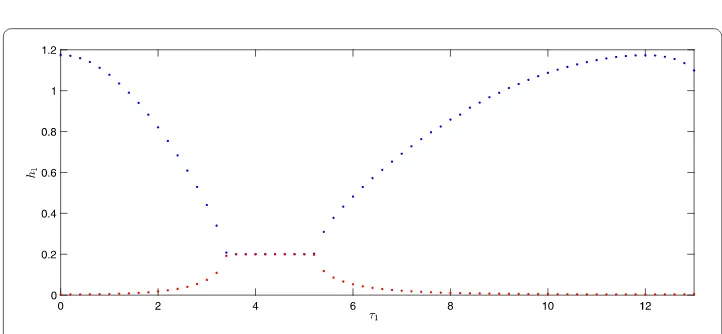
Example3 We chooseε= 1,κ= 2,μ= 0.17,d= 0.038,m= 0.05,τ1= 2. This leads to the case: 0 <A/2 <d<A. Ifτ1= 2 andm= 0, the coexistence equilibriumE2is unstable. As we takem= 0.05, we find there exists a stable interval asτ2increases, which is illustrated in Fig.3.
In order to investigate our model (2.2) in the cased>A> 0, two dispersal delays may induce Hopf bifurcation. Thus, we first plot the numerical solutions and theτ1-bifurcation
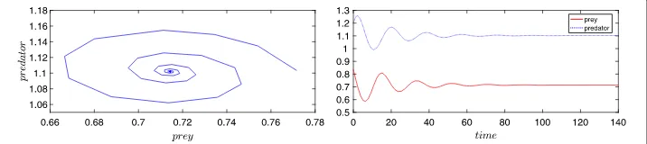
Figure 2The two figures show that the coexistence equilibriumE2is unstable with parameter valuesε= 1,
κ= 2,μ= 0.17,d= 0.0125,m= 0.02,τ1= 2,τ2= 2. System (2.2) has a periodic solution. Left panel: the phase graph of model (2.2) in each patch; right panel: the trajectory graph of model (2.2) in each patch
Figure 3Theτ2-bifurcation diagram of system (2.2) in the caseA/2 <d<A. Parameter values areε= 1,κ= 2,
μ= 0.17,d= 0.038,m= 0.05,τ1= 2
Figure 4 τ1-bifurcation diagram of system (2.2) under cased>Awith parameterε= 1,κ= 2,μ= 0.17, d= 0.1,m= 0
diagram of (2.2) withm= 0 in each cases. Then we choose values ofτ1in its stable intervals and unstable intervals, respectively. We regardτ2as bifurcation parameter and display the bifurcation diagram of (2.2).
Figure 5Bifurcation diagram of system (2.2) by regardingτ2as bifurcation parameter with parameter values
ε= 1,κ= 2,μ= 0.17,d= 0.1,m= 0.05. Left panel:τ1= 2; right panel:τ1= 6
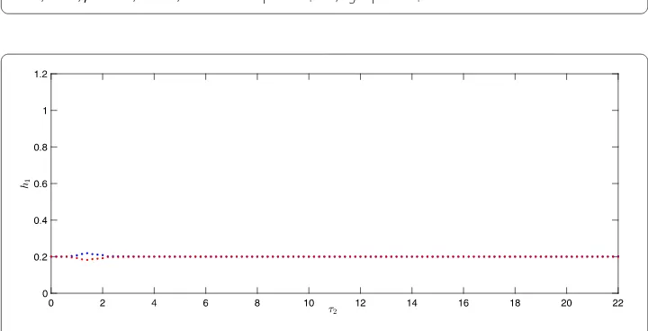
Figure 6 τ2-bifurcation diagram of system (2.2) withε= 1,κ= 2,μ= 0.17,d= 0.1,m= 1,τ1= 4
Next, we take two sets of parameter valuesm= 0.05,τ1= 2 andm= 0.05,τ1= 6, respec-tively, and keep all other parameter values the same as above. As we see in Fig.4,τ1= 2 and
τ1= 6, the system (2.2) is unstable at the coexistence equilibriumE2. We also investigate that the coexistence equilibrium is unstable ifm= 0.05,τ1= 2 andτ2= 0, while it is stable ifm= 0.05,τ1= 6 andτ2= 0. Asτ2increases, there is a stable interval which is illustrated in Fig.5.
Note that the coexistence equilibriumE2is stable whenτ1= 4 in Fig.4. Thus we finally take parameter valuesε= 1,κ= 2,μ= 0.17,d= 0.1,m= 1,τ1= 4, and present the bifur-cation diagram of system (2.2) by regardingτ2as bifurcation parameter (see Fig.6). We show that system (2.2) has a stable switch withτ1= 4 asτ2increases.
In all, as shown in Fig.5and Fig.6, dispersal delays may exhibit both stabilizing and destabilizing effects on the coexistence equilibrium.
5 Summary and discussion
dif-ficult. Numerical simulations are carried out showing that stability switches are possible. We leave the related analysis for our future work.
Acknowledgements
The authors wish to thank the editor and the referees for reading this manuscript.
Funding
This work was supported by the National Natural Science Foundation of China (No. 11371313 and No. 61573016) and by the Foundation of Yuncheng University (No. YQ-2017003 and No. YQ-2014011). AM was partially supported by China Scholarship Council (No. 201608140214).
Competing interests
The authors declare that they have no competing interests.
Authors’ contributions
All authors contributed equally to the writing of this paper. The authors read and approved the final manuscript.
Publisher’s Note
Springer Nature remains neutral with regard to jurisdictional claims in published maps and institutional affiliations.
Received: 24 August 2018 Accepted: 2 October 2018
References
1. Hanski, I.: Metapopulation dynamics. Nature396(6706), 41 (1998)
2. Shigesada, N., Kawasaki, K.: Biological Invasions: Theory and Practice. Oxford University Press, London (1997) 3. Pillai, P., Gonzalez, A., Loreau, M.: Evolution of dispersal in a predator–prey metacommunity. Am. Nat.179(2), 204–216
(2011)
4. Andersen, V., Gubanova, A., Nival, P., Ruellet, T.: Zooplankton community during the transition from spring bloom to oligotrophy in the open nw Mediterranean and effects of wind events. 2. Vertical distributions and migrations. J. Plankton Res.23(3), 243–261 (2001)
5. Freedman, H.I.: Single species migration in two habitats: persistence and extinction. Math. Model.8, 778–780 (1987) 6. Kuang, Y., Takeuchi, Y.: Predator–prey dynamics in models of prey dispersal in two-patch environments. Math. Biosci.
120(1), 77–98 (1994)
7. Kang, Y., Sourav, K.S., Komi, M.: A two-patch prey-predator model with predator dispersal driven by the predation strength. Math. Biosci. Eng.14(4), 843–880 (2017)
8. Zhang, Y., Lutscher, F., Guichard, F.: The effect of predator avoidance and travel time delay on the stability of predator–prey metacommunities. Theor. Ecol.8(3), 273–283 (2015)
9. El Abdllaoui, A., Auger, P., Kooi, B.W., De la Parra, R.B., Mchich, R.: Effects of density-dependent migrations on stability of a two-patch predator–prey model. Math. Biosci.210(1), 335–354 (2007)
10. Mchich, R., Auger, P., Poggiale, J.-C.: Effect of predator density dependent dispersal of prey on stability of a predator–prey system. Math. Biosci.206(2), 343–356 (2007)
11. Feng, W., Rock, B., Hinson, J.: On a new model of two-patch predator prey system with migration of both species. J. Appl. Anal. Comput.1(2), 193–203 (2011)
12. Kot, M.: Elements of Mathematical Ecology. Cambridge University Press, Cambridge (2001)
13. Cooke, K.L., Grossman, Z.: Discrete delay, distributed delay and stability switches. J. Math. Anal. Appl.86(2), 592–627 (1982)
14. Yang, K.: Delay Differential Equations: With Applications in Population Dynamics. Academic Press, New York (1993) 15. Wei, J., Ruan, S.: Stability and bifurcation in a neural network model with two delays. Phys. D, Nonlinear Phenom.
130(4), 255–272 (1999)