Application of a deep learning technique to the problem of oil spreading in the Gulf of Thailand

(1)

R E S E A R C H

Open Access

Application of a deep learning technique to

the problem of oil spreading in the Gulf of

Thailand

Polapat Khlongkhoi

1,2

_{, Kittisak Chayantrakom}

1,2*

_{and Wattana Kanbua}

3

*_{Correspondence:}

Full list of author information is available at the end of the article

Abstract

One of the important mechanisms of the oil weathering processes (OWP) is

spreading of oil spills. This mechanism is the horizontal expansion of the oil slick with inertia-gravity, gravity-viscosity, and viscous-surface tension. In the prediction of spreading, the surface of the slick can be considered as an ellipse where the major axis is in the direction of the wind. Ocean wave models, which account for the interaction between wind and waves, can be used to predict the state of the sea including wind direction in two dimensions where the wave spectrum is allowed to evolve freely with no constraints on the spectral shape. However, the wave model simulation for long duration is time-consuming. In this study, the technique of deep learning, a part of the machine learning method, is implemented to obtain a model used to get quick prediction of the wind direction. The technique uses outputs from an ocean wave model and applies the multivariate time series to obtain a linear relationship among multiple time series of wind prediction from the wave model. The wind forecast is taken as inputs to the deep learning model. Some of these inputs that are signiﬁcant are selected by using the sigmoid function which is an activation function. The minimum error of prediction from the deep learning model is obtained by the gradient descent method. The numerical results of the prediction spreading of oil spill in the Gulf of Thailand based on the wind prediction by the deep learning technique are presented.

Keywords: Deep learning; Gradient descent; Ocean wave model; Oil spill; Sigmoid function; Multivariate time series

1 Introduction

After crude oil leaks on the sea surface due to the crude oil exploration, crude oil trans-portation or accidents from the explosion of the oil rig, it can aﬀect and harm the envi-ronment for a long period of time. When crude oil spills into the sea, it can cause the oil weathering processes (OWP) [1] which produce natural, physical, and chemical changes. They are scattered in a thin layer called oil slicks.

A review of oil spill modeling, conducted by the American Society of Civil Engineers Task Committee on Modeling of Oil Spills (ASCE) [2], focuses on the oil spill processes for the real-time models, emergency planning, and risk assessment. When crude oil is spilled, protective measures need to be taken to reduce the impact. To take these measures, we

(2)

must be able to predict the short-term and long-term behavior of the oil spill using basic analytical techniques.

The input data required by oil spill models are wave height, wave direction, wind speed, and wind direction. These data can be obtained from ocean wave models, for example, the wave modeling (WAM) model. The WAM model was first developed by a group of researchers [3] in Norway in 1988. In this study, a technique of deep learning is imple-mented by using output data from the ocean wave model. This would improve accuracy and reduce time consumption in wave simulation based on the ocean wave model. In [4], Kanbua and Chuai-Aree studied the sea wave generated by tropical cyclones in the Gulf of Thailand. Their work was carried out by using the cycle 4 version of the WAM model. The model domain covered latitudes 5N–15N and longitudes 95E-105E, and the model spatial resolution reached 0.25 degree. The model can somewhat reproduce the observed characteristics of the waves. One of the widely used methods for simulating ocean waves is making use of wind-wave spectrums. The ocean waves produced in this way can reflect the statistical characteristics of the real ocean well. The waves just look like superposition of significant wave heights.

Many research works in deep learning have been carried out recently. Hossain et al. [5] compared the accuracy of historical pressure, humidity, and temperature data gathered from meteorological sensors in Northwestern Nevada and deep learning network with Stacked Denoising Auto-Encoders (SDAE). In 2016, Gupta et al. [6] compared the per-formance of two optimization techniques in the linear regression model for an accurate weather prediction.

2 Deep learning method

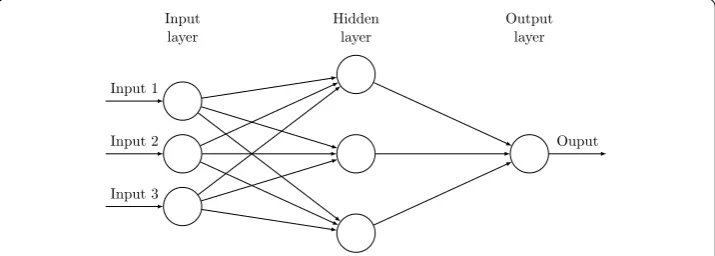
The artiﬁcial neurons which imitate the human brain neurons are the basic building blocks of neural networks. As shown in Fig.1, the processes in a neural network are described as follows. When input signals are weighted, they use an activation function to produce an output signal. These neurons are spread across several layers, including input layers, hid-den layers, and output layers, on the neural network. A connection between two neurons refers to the strength or amplitude, and it is called neuron weights. Usually, the weights are initialized by small random numbers ranging from 0 to 1. The neuron weights get updated when the network is trained to be more predictive. To control the inception of a neuron, an activation function is used to map summed weighted input to the output of the neuron.

(3)

For a pre-activation function, we use a multiple linear regression technique [7] as fol-lows:

g(x) = wTx+b, (1)

where grepresents a pre-activation function, x andb are input vector and bias values, and w is the vector of the connection weights which represent the strengths between the connections of neurons.

Next, we use the output from pre-activation function to compute activation function by

ˆ

y(x) =ag(x)=awTx+b, (2)

wherey(x) is the predicted output from neurons andˆ a(·) is the activation function. We use sigmoid activation function. This function gives a value between 0 and 1. The value is always positive, bounded, and strictly increasing. When the pre-activation func-tion gives the higher value, there is more chance the neuron is activated. The funcfunc-tion is given by

jk is the weight from thekth neuron in the (i– 1)th layer to thejth neuron in the

ith layer,bi

jandgjiare the bias and the pre-activation value of thejth neuron in theith

layer, respectively.

The cost function, which is derived from a loss function, is used to compute the error between the prediction and the actual data. Given (x(1)_,_y(1)_{), . . . , (x}(m)_,_y(m)_{), where}_x(i) _is

the actual input andy(i) _{is the actual output, we seek}_y_ˆ(i)_≈_y(i)_{. For this purpose, the loss}

function is utilized to compute the error for a single training example by measuring the discrepancy between the predictionyˆ(i)_{and the desired output}_y(i)_{. The cost function can}

be obtained using the loss functionL(yˆ(i)_,_y(i)_{) of the entire training set which is in the form}

of sum of squared errors (SSE):

Lyˆ(i),y(i)=1 2

ˆ

y(i)–y(i)2. (6)

The values of the connection weight w and the bias valueb can be found so that the overall cost functionJ(w,b) is minimized, where

(4)

We can reduce the value of the cost function by adjusting the weight values between the neurons. The weight values may be changed until the cost function is minimized. We use the technique called the gradient descent method to ﬁnd the minimum value of the cost function.

Letθ denote the parameters including the connection weights w and the bias valuesb. In the gradient descent method, the parameters are updated by

θj=θj–α

In this study, the input data include signiﬁcant wave height, wind speed, and wind di-rection. The data are divided into train data sets and test data sets using the ratio 2 to 1.

3 Models

3.1 Ocean wave model

The WAM model [8] is a third-generation wave model which is based on the wave trans-port equation. The model does not need a requirement on the shape of the wave spectrum. Therefore, the governing equation is the wave energy equation which is given by, at any speciﬁc location on the sea surface,

∂E

whereErepresents the spectral density such thatφ,λ,θ, andtare latitudes, longitudes, directions, and times, respectively.

The termsφ˙,λ˙, andθ˙are the rates of change of the position and propagation direction of a wave packet traveling along a great circle path.Sin is the wave energy inﬂux from

winds,Sdsdenotes the dissipation of wave energy, andSnlis the nonlinear eﬀects caused

by wind-wave interaction.

The model can be implemented for any given regional or global grid with a topographic data set. The wave propagation can be done on a latitudinal-longitudinal grid or on a Cartesian grid. The model yields various outputs including signiﬁcant wave height, mean wave direction and frequency, swell wave height and mean direction, and wind direction.

3.2 Oil-spill model

After oil is spilled on the sea surface, oil slicks can be aﬀected by the oil weathering pro-cesses (OWP). In [9], Fay described oil spreading, one process of OWP, as a horizontal expansion of the oil slick with inertia-gravity, gravity-viscous, and viscous-surface tension [2,10]. Lehr [11] considered that the oil spill can be spread in an elliptical shape whose major axis is in the direction of the wind [12,13]. The spreading equations are given by

(5)

Lmax=Lmin+ 0.95Uw4/3t3/4, (12)

A= 2270

ρ ρ0

2/3

V_oil2/3t1/2+ 40

ρ ρ0

1/3

V_oil1/3U_w4/3t, (13)

whereLminandLmaxare the lengths (m) of the minor and major axes of an ellipse,

respec-tively, andAis the area of oil slick (m2). The termsρw,ρ0are the densities of water and oil,

respectively, such thatρ=ρw–ρ0.Voildenotes the total volume of an oil spill in barrels,

Uwis the wind speed (knots) at 10 m over sea surface, andtis time (min.).

4 Numerical results

In this section, we present the simulation results of prediction of wind speed and direction in the movement of oil spill. The wind ﬁeld forecast including the wind speed and the wind direction is based on the deep learning technique. The wind prediction is then used for studying the spreading of oil spill.

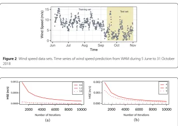
In this study, the outputs of wind data from WAM during 5 June to 31 October 2018 are used as a data set in the deep learning technique. The outputs are available every three hours each day, starting at 7.00 am (local time). There are totally 1,192 data points. Two thirds of the data set is taken as the training set, whereas one third of the data set is used as the test set as shown in Fig.2.

For the wind speed prediction, Figs.3(a) and3(b) show the plots of mean square errors (MSE) of wind speed versus the number of iterations of training where we investigate the suitable values of the learning rateαand the number of hidden layers, respectively. The results show that MSE is lower whenα= 1.2 and 3.0. Therefore,α= 1.2 is selected for our deep learning technique since there is no signiﬁcant diﬀerence resulting fromα= 3.0

Figure 2Wind speed data sets. Time series of wind speed prediction from WAM during 5 June to 31 October 2018

(6)

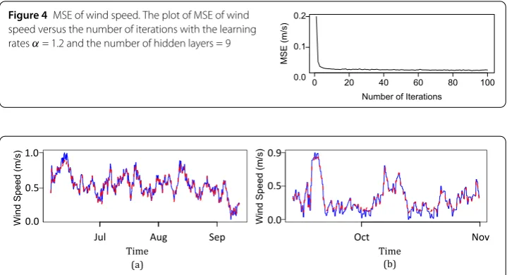
Figure 4MSE of wind speed. The plot of MSE of wind speed versus the number of iterations with the learning ratesα= 1.2 and the number of hidden layers = 9

Figure 5Deep learning prediction of wind speed. The plot of wind speed versus time (a) using the training set (blue solid line) and the deep learning technique (red dashed line) and (b) using the test set (blue solid line) and the deep learning technique (red dashed line)

Figure 6Wind direction data sets. Time series of wind direction prediction from WAM during 5 June to 31 October 2018

as shown in Fig.3(a). Moreover, MSE is lowest when the number of hidden layers is 9 as shown in Fig.3(b). As a result, the learning rate ofα= 1.2 and the number of hidden layers of 9 are used in the prediction model obtained from the deep learning technique.

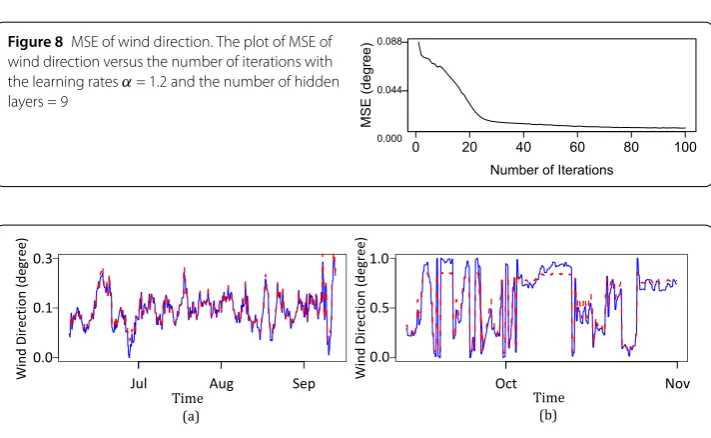
Figure4shows the plot of MSE of wind speed versus the number of iterations. It can be seen that MSE decreases when the model is run through more iterations. Figures5(a) and5(b) present the plots of wind speed versus time for the training set and the test set, re-spectively, using the predictive model. It can be seen that the model gives good prediction. For the wind direction prediction, the results follow in the same manner as those of the wind speed prediction, as shown in Figs.6–9.

To investigate the computing time used in the deep learning technique against the num-ber of iterations, we divide the data set into groups. The results show that when 50 or 100 iterations are applied, the computing time decreases very fast when we divide the data set into more groups, as shown in Tables1–2.

(7)

Figure 7MSE of wind direction (learning rates and hidden layers). The plot of MSE of wind direction versus the number of iterations (a) with various learning rates:α= 0.5 (solid line),α= 1.2 (dashed line), andα= 3.0 (dotted line) and (b) with various numbers of hidden layers of 4 (solid line), 6 (dashed line), and 9 (dotted line)

Figure 8MSE of wind direction. The plot of MSE of wind direction versus the number of iterations with the learning ratesα= 1.2 and the number of hidden layers = 9

Figure 9Deep learning prediction of wind direction. The plot of wind direction versus time (a) using the training set (blue solid line) and the deep learning technique (red dashed line) and (b) using the test set (blue solid line) and the deep learning technique (red dashed line)

Table 1 Comparison of computing time in wind speed prediction using various numbers of

iterations and numbers of data groups

Number of iterations

Number of data groups

1 5 10 20

10 Training set MSE 0.000430 0.000346 0.000370 0.000536 Test set MSE 0.000463 0.000454 0.000520 0.000838 Time (min.) 0.987254 0.308509 0.246547 0.207704

5 Conclusions

(8)

predic-Table 2 Comparison of computing time in wind direction prediction using various numbers of iterations and numbers of data groups

Number of iterations

Number of data groups

1 5 10 20

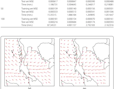
Figure 10 Oil spill spreading. The prediction of oil spill spreading at timetandt+ 1 on 6 December 2018 using the wind prediction (a) from the ocean wave model and (b) from the deep learning technique

tion model. The results show that the model can give good prediction on wind speed and direction with high accuracy when the learning rate is 1.2 and the number of hidden lay-ers is 9. Furthermore, the prediction on the spreading of oil spill using the wind prediction from the deep learning technique agrees with that from the WAM model, while the deep learning technique takes less computing time on wind prediction.

Acknowledgements

We would like to thank Thai Marine Meteorological Center, Thai Meteorological Department for providing the prediction data from WAM.

Funding

This research was ﬁnancially supported by the Centre of Excellence in Mathematics, Commission on Higher Education, Thailand.

Competing interests

The authors declare that they have no competing interests.

Authors’ contributions

(9)

Author details

1_{Department of Mathematics, Faculty of Science, Mahidol University, Bangkok, Thailand.}2_{Centre of Excellence in}

Mathematics, CHE, Bangkok, Thailand. 3_{Thai Marine Meteorological Center, Thai Meteorological Department, Bangkok,}

Thailand.

Publisher’s Note

Springer Nature remains neutral with regard to jurisdictional claims in published maps and institutional aﬃliations.

Received: 8 February 2019 Accepted: 15 July 2019

References

1. Sebastiao, P., Soares, C.G.: Modeling the fate of oil spills at sea. Spill Sci. Technol. Bull.2, 121–131 (1995) 2. ASCE Task Committee: State-of-the-art review of modeling transport and fate of oil spills. J. Hydraul. Eng.122,

594–609 (1996)

3. Hasselmann, S., Hasselmann, K., Janssen, P.A.E.M., Bauer, E., Komen, G.J., Bertotti, L., Lionello, P., Guillaume, A., Cardone, V.C., Greenwood, J.A., et al.: The WAM model—a third generation ocean wave prediction model. J. Phys. Oceanogr. 18, 1775–1810 (1988)

4. Kanbua, W., Chuai-Aree, S.: Virtual wave: An algorithm for visualization of ocean wave forecast in the Gulf of Thailand. KMITL Sci. J.5, 140–150 (2005)

5. Hossain, M., Rekabdar, B., Louis, S.J., Dascalu, S.: Forecasting the weather of Nevada: a deep learning approach. In: 2015 International Joint Conference on Neural Networks (IJCNN) (2015)

6. Gupta, S., K, I., Singhal, G.: Weather prediction using normal equation method and linear regression techniques. Int. J. Comput. Sci. Inf. Technol.7(3), 1490–1493 (2016)

7. James, G., Witten, D., Hastie, T., Tibshirani, R.: An Introduction to Statistical Learning: With Applications in R. Springer, New York (2013)

8. Gunther, H., Hasselmann, K., Janssen, P.A.E.M.: Report NO.4, the WAM Model Cycle 4. Modellberatungsgruppe (ed.). Hamburg (1992)

9. Fay, J.A.: Physical processes in the spread of oil on a water surface. Int. Oil Spill Conf. Proc.1971(1), 463–467 (1971) 10. Shen, H.T., Yapa, P.D.: Oil slick transport in rivers. J. Hydraul. Eng.114, 529–543 (1988)

11. Lehr, W.J., Cekirge, H.M., Fraga, R.J., Belen, M.S.: Empirical studies of the spreading of the oil spills. Oil Petrochem. Pollut.2, 7–12 (1984)

12. Chao, X., Shankar, J., Cheong, H.F.: Two- and three-dimensional oil spill model for coastal waters. Ocean Eng.28, 1557–1573 (2001)