3-D coseismic displacement field of the 2005 Kashmir earthquake inferred
from satellite radar imagery
Hua Wang1, Linlin Ge2, Caijun Xu1, and Zhixing Du3
1School of Geodesy and Geomatics, Wuhan University, 129 Luoyu Road, Wuhan 430079, China
2School of Surveying&Spatial Information Systems, The University of New South Wales, Sydney NSW 2052, Australia 3Geoinformation Science & Engineering College, Shandong University of Science and Technology, China
(Received October 18, 2006; Revised January 10, 2007; Accepted January 17, 2007; Online published June 8, 2007)
We use radar amplitude images acquired by the ENVISAT/ASAR sensor to measure the coseismic deformation of the 8 October 2005 Kashmir earthquake. We use the offset images to constrain the fault trace, which is in good agreement with field investigations and aftershock distribution. We infer a complete 3-D surface displacement field of the Kashmir earthquake using the offset measurements derived from both descending and ascending pairs of SAR images. The peak-to-peak offsets are up to (3.9, 3.6, 4.1) m in the east, north, and up directions respectively, i.e., 2.9 and 4.1 m along and across the fault assuming striking 325◦. We model the coseismic displacements using a four-segment dislocation model in a homogeneous elastic half-space. We first estimate the source parameters using a uniform slip model. Then we fix the optimal geometric parameters and solve for the slip distribution using a bounded variable least-squares (BVLS) method. The resultant maximum slip is about 9.0 m at depth of 4–8 km beneath Muzaffarabad. We find a scalar moment of 2.34×10²⁰N m (M
w7.55), of which almost 82% is released in the uppermost 10 km.
Key words:Kashmir earthquake, offset, 3-D displacement, slip distribution.
1.
Introduction
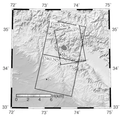
The 8 October 2005 Kashmir earthquake occurred on the Muzaffarabad fault where the Indian plate subducts under the Eurasian plate and is moving northward at a rate of about 40 mm/a. The collision between these two continen-tal plates fractured the northern boundary of Indian plate into several slices beneath the Kashmir Basin, known as the Indus-Kohistan seismic zone (IKSZ) (Seeber and Arm-bruster, 1979). IKSZ is a seismically active zone and a Mw>8 earthquake was predicted in this area through pre-vious studies before the occurrence of the Kashmir earth-quake (Bilham et al., 2001; Bilham and Wallace, 2005). Figure 1 shows the topographic setting and radar imaging geometry for the Kashmir earthquake. The moment magni-tude of the major shock is aboutMw7.6, with its epicenter at (34.476◦N, 73.577◦E), about 19 km NE of Muzaffarabad, and 105 km NNE of Islamabad, Pakistan (U.S. Geologi-cal Survey Earthquake Hazards Program, 2005). More than 79,000 people were killed, 83,000 injured, and 2.5 million left homeless in the disaster. It is the largest devastating event in the Kashmir area over the past 100 years.
Parsonset al.(2006) analyzed the coseismic static stress changes associated with the Kashmir earthquake from tele-seismic body waveforms (P-wave). The remote sensing techniques, e.g. interferometric synthetic aperture radar (In-SAR), play an important role for the prompt analysis of the earthquake. Fujiwaraet al.(2006) generated a range offset
Copyright cThe Society of Geomagnetism and Earth, Planetary and Space Sci-ences (SGEPSS); The Seismological Society of Japan; The Volcanological Society of Japan; The Geodetic Society of Japan; The Japanese Society for Planetary Sci-ences; TERRAPUB.
(RO) map with ENVISAT/ASAR data from a descending orbit to identify the fault trace, and estimated the source pa-rameters using a uniform slip dislocation model. Wright and Pathier (2005) also identified the fault trace using the RO map 1 month after the seismic event. In this study, we will infer a complete 3-D displacement field of the Kashmir earthquake using more radar images from both descending and ascending orbits. Based on the amplitude offset mea-surements, we will estimate the slip distribution on the fault plane for the earthquake.
2.
Data Analysis
2.1 Azimuth and range offsets of radar amplitude
im-ages
To support the studies on the devastating Kashmir earth-quake, ESA released 11 scenes of radar images acquired by the ENVISAT/ASAR sensor just 2 weeks after the seis-mic event. Among them, eight scenes were acquired from a descending orbit and three scenes from an ascending or-bit. For either orbit, only one image was acquired after the earthquake. Table 1 is the list of the interferometric pairs used in this study.
We process the radar data using the two-pass InSAR method (Massonnetet al., 1993). Although only spanning a time interval of 35 days for IP1 and IP2, they are still almost completely decorrelated in the epicentral area. The decor-relation may be ascribed to large-scale surface fissuring and landslides after the major shock besides the rough terrain and the long perpendicular baselines.
In contrast to the interferometric approach, the azimuth and range offset approach has at least three advantages: (1)
Fig. 1. Shaded relief map of the epicentral area of the Kashmir earthquake. Data shown are 3 arc-second DEM data from the SRTM (Farr and Ko-brick, 2000). Pre-existing fault locations are shown with a dashed line (Kumahara and Nakata, 2006). Solid squares denote ENVISAT/ASAR scenes from the descending (track 2463, frames 2907 and 2925) and the ascending (track 6499, frame 675) orbits. White arrows indicate the satellite look direction (ground to satellite). Islamabad (IS) and Muzaf-farabad (MU) are indicated as black triangles. The circles in red-white color denote the Harvard CMT solution of the major event (Mw7.6).
Table 1. Interferometric pairs used in this study.
Direction Interferometric Pair B⊥a Tb
(year/month/day) (m) (day)
DSCc 20050709–20051022 −456 105
DSC 20050813–20051022 606 70
DSC 20050917–20051022 (IP1) 297 35
ASCd 20050815–20051024 990 70
ASC 20050919–20051024 (IP2) 296 35
aB
⊥: perpendicular baselinebT: temporal baselinecDSC: descending, track 2463, frames 2907 and 2925dASC: ascending, track 6499, frame 675
it is less sensitive to coherence, (2) phase unwrapping is not required, and (3) displacements near the epicentral area are obtainable, so that the fault location can be clearly identified (e.g. Peltzeret al., 1999). What’s more, offset estimation of ASAR data can even achieve accuracies of up to 1/50 pixel in range and azimuth directions, i.e., 14 cm and 7.5 cm, respectively (Werneret al., 2005). Therefore, it is useful for monitoring large magnitude deformation (e.g. Michelet al., 1999a,b; Tobitaet al., 2001).
In this study, we first estimate range and azimuth offsets for each grid with 6 arc-second spacing using the intensity cross-correlation method. A quadratic polynomial trend is then removed from the estimations in each offset image in order to mitigate the systematic offset due to orbit errors. Finally, the offset value on the reference point is subtracted from all estimations in each offset image. Figure 2 shows the resultant range and azimuth offset images for IP1 and IP2 with 6 arc-second spacing. The descending azimuth offset (AZO) image shows positive values on the NE side of the fault; in contrast, the ascending one shows negative values on this side. The difference is mainly due to the dif-ferent flight direction of the satellite (see arrows in Fig. 1). We can clearly identify the seismic fault location from these
and Nakata, 2006) and the aftershock distribution denoted as small open circles in Fig. 2.
Figure 2(e)–(f) show the profiles averaged in a 20-km bin along line A. The profiles show a good agreement of the rupture location between descending and ascending off-set images. The peak-to-peak offoff-sets are about 3.9 m in range and 4.8 m in the azimuth direction in the descending images, whereas, they are about 4.8 m and 3.9 m, respec-tively, in the ascending images. The magnitude differences are mainly due to the different flight directions of the satel-lite in the descending and ascending orbits.
2.2 3-D offset maps
Since we have obtained both RO and AZO images from different satellite flight directions, the 3-D displacement field of the Kashmir earthquake can be determined. We fol-low the method described by Fialkoet al.(2001) and Wright et al. (2004). Suppose that the vectoru = [ue un uu]T
represents three orthogonal components of displacements in the local coordinate system (e.g. east, north, and up),
d = [dr daz]T represents displacements in range and
az-imuth directions. If they belong to the same reference frame, the transformation formula fromutodcan be ex-pressed as
d=s·u, (1)
wheresis the unit vector.
s=
whereαis the azimuth of the satellite heading vector (pos-itive clockwise from the north), and θ is the radar inci-dence angle at the reflection point. Customarily we define upwards as positive foruu, whereas increases in the radar
range are positive fordr. This is the reason that the signs in
Eq. 2 are different from Fialkoet al.(2001).
Given displacements acquired from no less than three directions in different planes, a complete 3-D displacement field can be inverted by the least-squares method,
u=(sTPs)−1sTPd, (3)
wherePis the weight matrix for the observations.
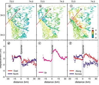
Based on the above model, the 3-D displacement field for the Kashmir earthquake is inverted from four RO and AZO images obtained previously (Fig. 3(a)–(c)). Profiles for Line A in the ENU directions are obtained using the same method as that for Fig. 2. Furthermore, they are projected along and across the fault given striking 325◦. The peak-to-peak values are about (3.9, 3.6, 4.1) m in the ENU directions, respectively, and they are about 2.9 m and 4.1 m along and across the fault, respectively. Our observations are in agreement with earlier results indicating the oblique (reverse and right-lateral) sense of motion on the Muzaffarabad fault (Nakataet al., 1991).
3.
Modeling
3.1 Data reduction and weighting
Fig. 2. (a) RO and (b) AZO images from the descending orbit (c) RO and (d) AZO images from the ascending orbit (e) the profiles for Line A from the descending orbit (f) The profiles for Line A from the ascending orbit. The solid blue line in (a)–(d) represents the fault identified from the offset images. The dashed red line in (a)–(d) represents the seismic fault from field investigations (Kumahara and Nakata, 2006). The numbers in the white rectangles on the blue line denote the segment number for fault modeling. The small open circles denote the aftershocks (from Harvard CMT). The red cross located at (34◦N, 73◦33E) denotes the reference point.
Fig. 3. Complete 3-D coseismic displacement field of the Kashmir earthquake. (a)–(c) Displacements of east, north and up components. (d)–(f) Profiles for Line A in the east, north, and up directions, and their projections along and across the fault given striking 325◦.
data. We reduce the data using a quadtree algorithm (e.g. J´onsson et al., 2002; Simonset al., 2002). The algorithm divides the whole image into quadrants and then calculates the root-mean-square (RMS) in each quadrant. If the RMS exceeds a given threshold, e.g. 0.2 pixels in this study, the quadrant is further subdivided into four. Otherwise, the average value in the quadrant is the output. This process
(%) (cm) (Nm)
aσ: RMS values for the distributed slip model. bM0: scalar moments for the distributed slip model.
boundaries in the deformation maps (Masterlark and Lu, 2004). Using the above strategies, only 2313 data points are left in the down-sampled data sets (Table 2).
To ensure a balanced contribution of different data sets in a joint inversion, reasonable weights should be assigned to the observations. In this study, we use similar weighting strategies as Fialko (2004). Within a particular data set, the weight ratio of an individual point is proportional to the quadrant size during down-sampling. Among the data sets, a ratio is given to each data set to keep a balance of residuals. The resultant weight for each data point is expressed in Eq. (4), and the sum of weights equals unity, i.e., Eq. (5).
data set; Nj is the number of the data points in the jth
data set; σ2 is the variance of the data points; n is the quadrant size from quadtree sampling;βjis the weight ratio
for the jth data set; Nf is the number of data sets. In
this study, we set the ratio 36% to the descending RO and AZO images, 18% and 10% to the ascending AZO and RO images, respectively.
3.2 Fault slip distribution
We first estimate the fault geometry using a uniform slip model in a homogeneous elastic half-space (Okada, 1985). We find that four fault segments can reasonably represent the fault trace (see Fig. 2 for each segment indication). The surface displacements are nonlinear functions of the fault geometry, so we use a genetic algorithm (GA) to determine the optimal model which minimizes the weighted misfits between the observations and the modeled values (Carroll, 1996). We assume the top edges intersect the surface. The rake is constrained between 90◦ and 180◦ for right-lateral strike slip (Aki and Richards, 2002). The other parameters are left free during inversion. The inverted source parame-ters are listed in Table 3. The maximum slip is 6.0 m and occurred on the third segment NW of the epicenter. It is a bit smaller than that in Fujiwaraet al.(2006) who only used the descending range changes. We have also obtained
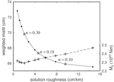
Fig. 4. Tradeoff between weighted misfit and solution roughness for the distributed slip model. Stars indicate the smoothing factors (κ=0.10,0.18,0.30) used in the inversions shown in Fig. 5.
similar results while only using the descending RO image. We believe it is more reliable to model the fault with both descending and ascending images since the slip really oc-curred in a 3-D space. The average strike is 328◦ and dip is 34◦, similar to Fujiwaraet al.(2006) and Parsonset al. (2006). The resultant moment tensorM0is 2.19×10²⁰N m
(Mw7.53), assuming Lam´e constantsμ=λ=33 GPa. To obtain slip distribution, the width of the fault is ex-tended to 30 km, and the length is increased by 10 km for segments 1 and 4 to account for the whole fault plane in the model. The fault plane is then discretized into 310 patches each with a size of 3×3 km. We fix the geometric param-eters from the uniform slip model and solve for the optimal slip on each patch. The surface displacements are then the linear functions of dislocations. To determine such a slip model, we set up the following equations:
wheredis a vector containing the observed displacements;
Gis a matrix containing Green’s functions (e.g., Okada, 1985);∇2is a second-order finite difference approximation of the Laplacian operator and the Lagrange multiplierκ2
that determine the weight of smoothing (Harris and Segall, 1987);His a matrix containing the coordinates of the data points;tis a vector containing the bilinear ramp coefficients to correct the orbit errors.
We solve the system of Eq. 6 using a bounded variable least-squares (BVLS) method (Stark and Parker, 1995), which can seek the bounded variables to minimize the ob-jective function (Eq. (7)).
= W(d−Gm−Ht)L2+ κ2∇2mL2 (7)
where W is the matrix from Cholesky decomposition of weight matrixP, i.e., WTW = P. In this study, we con-strain the right-lateral strike-slip components to the range from 0 to 9 m and the dip-slip components from 0 to 10 m. Because the best-fit slip distribution depends on the smoothing factor κ2, we show the tradeoff between
Table 3. Uniform slip model inverted from the offset imagesa.
No. Slip x0 y0 Length Width Strike Dip Rake
(m) (km) (km) (km) (km) (◦) (◦) (◦)
1 3.8 −41.8 31.0 19.7 10 333 23 92
2 5.5 −25.3 20.3 33.3 15 326 35 91
3 6.0 0.9 −0.3 9.5 23 315 42 112
4 5.4 8.3 −6.3 16.0 21 338 35 115
aCoordinatesx0,y
0correspond to the top-right corner of each segment. The top edges are assumed to inter-sect the surface. Origin is taken to be at the epicenter of the Kashmir earthquake (34.37N, 73.47E) (Harvard CMT).
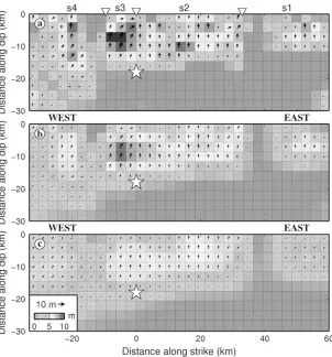
Fig. 5. Slip distribution for different smoothing factors: (a)κ=0.10, (b)κ=0.18, (c)κ=0.30. We pick the second as the resultant model because of its good compatibility between weighted misfit and solution roughness. The numbers between the triangles in (a) indicate the segments. The white star denotes the epicenter from Harvard CMT solution.
and solution roughness (Fig. 5). The scalar moment does not change too much for different smoothing factors, which ranges 2.3∼2.5×10²⁰ N m from Fig. 4. We find the re-sultant moment of 2.34×10²⁰ N m (Mw 7.55), which is similar to the Harvard CMT solution (2.94×10²⁰N m). Up to 82% of the energy is released in the uppermost 10 km. In Fig. 5(b), we find a maximum slip of 9.0 m at depth of 4–8 km, i.e.∼6–12 km along dip. Fault slip focused on the sec-ond and third segments in the uppermost 10 km. The main asperity in Fig. 5(b) located almost exactly beneath Muzaf-farabad, above the hypocenter from the Harvard CMT solu-tion.
In general, the slip distribution is in agreement with the result derived by Avouacet al.(2006) from the joint inver-sion of seismic waveforms and offset measurements with ASTER images. The difference is that their model shows more slip on the SE side of Muzaffarabad than that on the
NW side. In particular, almost all slip focuses on the SE side derived from the seismic waveforms data alone in their model. Since the maximum displacement from the ASTER measurements locates on the NW side, the inversion only using ASTER measurements may show a similar pattern to our model. The slip distribution pattern is also consistent with the one described in Pathieret al.(2006), who used a similar method to this study. The maximum slip (9.6 m) and moment tensor (3.36×10²⁰N m) in Pathieret al.(2006) are
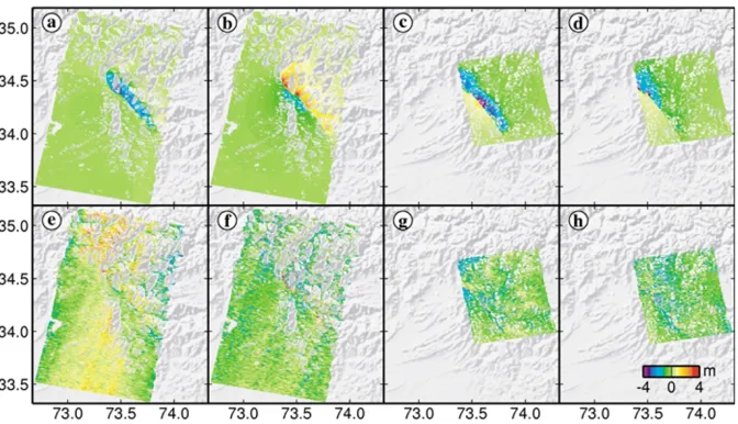
Fig. 6. Synthetic (a) RO and (b) AZO from the descending orbit, synthetic (c) RO and (d) AZO from the ascending orbit (e) RO and (f) AZO residuals from the descending orbit (g) RO and (h) AZO residuals from the ascending orbit. All the synthetic displacements are deduced from the distributed slip model in Fig. 5b.
4.
Discussion and conclusions
The 2005 Kashmir earthquake is the latest devastating seismic event that has occurred in the Himalayan zone. Be-cause of the steep topography in the epicentral area and the long baselines, it is almost impossible to obtain an ideal interferogram. Nevertheless we processed the EN-VISAT/ASAR data only 1 month after the event and ob-tained the azimuth and range offset images. The location of the fault was identified from the offset images. It is in good agreement with the field investigations and the after-shock distribution. This capability of SAR offset images for detecting seismic fault locations may play an important role for the near real-time estimation of damaged areas and prompt rescue in the future.
We have inferred a complete 3-D surface displacement field for the Kashmir earthquake using range and azimuth offset images acquired from descending and ascending pairs of SAR images. The peak-to-peak surface displace-ment is up to 4.1 m across the fault, 2.9 m along the fault, and 4.1 m upwards. In the future, the complete 3-D defor-mation monitoring using InSAR and its byproducts may be a routine procedure by combination of data acquired from multi-squint mode and different sensors.
We have modeled the fault slip distribution in a homo-geneous elastic half-space. The maximum slip is 9.0 m at a depth of 4–8 km beneath Muzaffarabad. The estimated geodetic moment is 2.34×10²⁰ N m (Mw7.55). It is still not clear whether the Kashmir earthquake is just an aus-pice for large earthquake sequences in the Himalayan zone (Bilhamet al., 2001; Bilham and Wallace, 2005). More at-tention should be paid for the monitoring and study in this area.
Acknowledgments. We thank the Associate Editor Dr. Takeshi Sagiya, Dr. Takuya Nishimura and an anonymous reviewer for their detailed and constructive reviews of the manuscript. We thank Dr. Yasuhiro Kumahara, Dr. Takashi Nakata and Dr. Yuzo Ishikawa for providing the Pakistan fault trace by field investiga-tions. The European Space Agency is gratefully acknowledged
for providing ENVISAT/ASAR imagery free of charge. All fig-ures in this study are prepared using GMT software (Wessel and Smith, 1998). This work was supported by Research Fund for the Program for New Century Excellent Talents in University (NCET-04-0681), a Specialized Research Fund for the Doctoral Program of Higher Education (No. 20030486038), the Nature and Science Fund of Qingdao (No. 04-2-JZ-101), and the foundation of LO-GEG State Bureau of Surveying and Mapping (No: 04-01-08).
References
Aki, K. and P. G. Richards,Quantitative Seismology, second edn, Univer-sity Science Books, Sausalito, CA, 2002.
Avouac, J.-P., F. Ayoub, S. Leprince,et al., The 2005,Mw7.6 Kashmir earthquake: Sub-pixel correlation of ASTER images and seismic wave-forms analysis,Earth Planet Sci. Lett.,249, 514–528, 2006.
Bilham, R. and K. Wallace, FutureMw>8 earthquakes in the Himalaya: Implications from the 26 Dec 2004Mw = 9.0 earthquake on India’s eastern plate margin,Geol. Surv. India Spl.,85, 1–14, 2005.
Bilham, R., V. K. Gaur, and P. Molnar, Himalayan seismic hazard,Science, 293, 1442–1444, 2001.
Carroll, D. L., Genetic algorithms and optimizing chemical Oxygen-Iodine Lasers, inDevelopments in Theoretical and Applied Mechanics, edited by H. B. Wilson, R. C. Batra, C. W. Bertet al., XVIII, School of Engineering, The University of Alabama, pp. 411–424, 1996. Farr, M. and M. Kobrick, Shuttle Radar Topography Mission produces a
wealth of data,EOS Trans.,81, 583–585, 2000.
Fialko, Y., Probing the mechanical properties of seismically active crust with space geodesy: Study of the co-seismic deformation due to the 1992Mw7.3 Landers (southern California) earthquake, J. Geophys. Res.,109(B03307), doi:10.1029/2003JB002756, 2004.
Fialko, Y., M. Simons, and D. Agnew, The complete (3-D) surface dis-placement field in the epicentral area of the 1999Mw7.1 Hector Mine earthquake, California, from space geodetic observations,Geophys. Res. Lett.,28(16), 3063–3066, 2001.
Fujiwara, S., M. Tobita, H. P. Sato,et al., Satellite data give snapshot of the 2005 Pakistan earthquake,EOS Trans.,87(7), 73–77, 2006. Harris, R. A. and P. Segall, Detection of a locked zone at depth on the
Parkfield, California, segment of the San Andreas fault,J. Geophys. Res.,92(B8), 7945–7962, 1987.
J´onsson, S., H. Zebker, P. Segall,et al., Fault slip distribution of the 1999
Mw7.1 Hector Mine, California, earthquake, estimated from satellite radar and GPS measurements,B. Seismol. Soc. Am.,92(4), 1377–1389, 2002.
Lasserre, C., G. Peltzer, F. Cramp´e, et al., Coseismic deformation of the 2001 Mw = 7.8 kokoxili earthquake in tibet, measured by syn-thetic aperture radar interferometry, J. Geophys. Res., 10(B12408), doi:10.1029/2004JB003500, 2005.
Massonnet, D., M. Rossi, C. Carmona,et al., The displacement field of the Landers earthquake mapped by radar interferometry,Nature,364, 138–142, 1993.
Masterlark, T. and Z. Lu, Transient volcano deformation sources im-aged with interferometric synthetic aperture radar: Application to Seguam Island, Alaska,J. Geophys. Res.,109(B01401), doi:10.1029/ 2003JB002558, 2004.
Michel, R., J.-P. Avouac, and J. Taboury, Measuring ground displacement from SAR amplitude images: application to the Landers earthquake,
Geophys. Res. Lett.,26(7), 875–878, 1999a.
Michel, R., J.-P. Avouac, and J. Taboury, Measuring near field coseismic displacement from SAR images: Application to the Landers earthquake,
Geophys. Res. Lett.,26(19), 3017–3020, 1999b.
Nakata, T., H. Tsutsumi, S. H. Khan,et al., Active faults of Pakistan, 141 pp., Res. Cent. for Reg. Geogr., Hiroshima Univ., Hiroshima, Japan, 1991.
Okada, Y., Surface deformation due to shear and tensile faults in a half-space,B. Seismol. Soc. Am.,75(4), 1135–1154, 1985.
Parsons, T., R. S. Yeats, Y. Yagi, et al., Static stress change from the 8 October, 2005 M = 7.6 Kashmir earthquake,Geophys. Res. Lett., 33(L06304), doi:10.1029/2005GL025429, 2006.
Pathier, E., E. J. Fielding, T. J. Wright,et al., Displacement field and slip distribution of the 2005 kashmir earthquake from SAR imagery,
Geophys. Res. Lett.33(L20310), doi:10.1029/2006GL027193, 2006. Peltzer, G., F. Cramp´e, and G. King, Evidence of the nonlinear elasticity of
the crust fromMw7.6 Manyi (Tibet) earthquake,Science,286, 272–276,
1999.
Seeber, L. and J. G. Armbruster, Seismicity of the Hazra arc in northern Pakistan: Decollement vs. basement faulting, inGeodynamics of Pak-istan, edited by A. Farah and K. A. DeJong, Geological Survey of Pak-istan, Quetta, pp. 131–142, 1979.
Simons, M., Y. Fialko, and L. Rivera, Coseismic deformation from the 1999Mw 7.1 Hector Mine, California, earthquake as inferred from InSAR and GPS observations,B. Seismol. Soc. Am.,92(4), 1390–1402, 2002.
Stark, P. B. and R. L. Parker, Bounded variable least squares: an algorithm and applications,Computational Statistics,10, 129–141, 1995. Tobita, M., M. Murakami, H. Nakagawa,et al., 3-D surface deformation of
the 2000 Usu eruption measured by matching of SAR images,Geophys. Res. Lett.,28(22), 4291–4294, 2001.
U.S. Geological Survey Earthquake Hazards Program, Magnitude 7.6 -PAKISTAN - usdyae, http://earthquake.usgs.gov/eqcenter/eqinthenews/ 2005/usdyae/, 2005.
Werner, C., U. Wegm¨uller, T. Strozzi,et al., Precision estimation of local offsets between pairs of SAR SLCs and detected SAR images, Interna-tional Geoscience and Remote Sensing Symposium, Seoul, Korea, 2005. Wessel, P. and W. H. F. Smith, New, improved version of generic mapping
tools released,EOS Trans.,79(47), 579, 1998.
Wright, T. and E. Pathier, Locating the Kashmir fault, http://comet.nerc.ac. uk/news kashmir.html, 2005.
Wright, T. J., B. E. Parsons, and Z. Lu, Toward mapping surface deforma-tion in three dimensions using InSAR,Geophys. Res. Lett.31, L01607, doi:10.1029/2003GL018827, 2004.