R E S E A R C H
Open Access
New mathematical model of vertical
transmission and cure of vector-borne
diseases and its numerical simulation
Abdullah
1, Aly Seadawy
2,3*and Wang Jun
1*Correspondence:
2Mathematics Department, Faculty
of Science, Taibah University, Al-Madinah Al-Munawarah, Saudi Arabia
3Mathematics Department, Faculty
of Science, Beni-Suef University, Beni-Suef, Egypt
Full list of author information is available at the end of the article
Abstract
In this research article, a new mathematical model for the transmission dynamics of vector-borne diseases with vertical transmission and cure is developed. The non-negative solutions of the model are shown. To understand the dynamical behavior of the epidemic model, the theory of basic reproduction number is used. As this number increases, the disease invades the population and vice versa. The effect of vertical transmission and cure rate on the basic reproduction number is shown. The disease-free and endemic equilibria of the model are found and both their local and global stabilities are presented. Finally, numerical simulations are carried out graphically to show the dynamical behaviors. These results show that vertical transmission and cure have a valuable effect on the transmission dynamics of the disease.
Keywords: Vector-borne disease; Vertical transmission; Cure; Stability; Numerical simulation
1 Introduction
Vector-borne diseases are infectious diseases transmitted to humans and animals by blood-feeding arthropods. Some common vector-borne diseases are West Nile virus, dengue fever, Rift Valley fever, malaria, and viral encephalitis caused by pathogens such as bacteria, viruses, and parasites. The arthropods are blood sucking insects and arach-nids such as ticks, mosquitoes, biting flies, and lice called vectors [1]. The vectors re-ceive pathogens from an infected host and transmit them to a human host, as humans are the major host, or animals. However, direct transmissions, such as transplantation related transmission, transfusion related transmission, and needle-stick-related transmis-sion, are also possible [2]. In case of some diseases such as AIDS and Hepatitis B, it is possible for the offspring of infected parents to be born infected. This type of transmis-sion is called vertical transmistransmis-sion. Now it is found that vector-borne diseases can also be transmitted vertically [3, 4]. Also new research shows that virus is transmitted from female mosquitos to their eggs at a high rate [5], which causes vertical transmission of the disease.
Vector-borne diseases are prevalent in hot areas, such as tropics and subtropics, and are relatively rare in temperate zones. Vector-borne infectious diseases remain amongst the
most important cause of global health illness and are major killers, particularly of children. The World Health Organization reports the numbers of deaths in different regions of the world annually. Nearly 700 million people get mosquito-borne illnesses that cause about one million deaths each year. Worldwide, malaria is the leading cause of premature mor-tality, particularly in children under the age of five. Nearly half of the world’s population is at risk of malaria, and every year 198 million cases (uncertainty range: 124–283 million) and 584,000 deaths (range: 367,000–755,000) occur according to the World Malaria Re-port 2014 [6]. According to WHO, an estimated of 3.3 billion people in 97 countries are at risk of malaria. Currently, dengue threatens up to 40% of the world’s population, and there may be 50–100 million infections annually [7]. More than 2.5 billion people over 40% of the world’s population are now at risk of dengue.
From the above discussion it is clear that it is necessary to control such epidemic diseases. Control measures for vector-borne diseases are important because most are zoonoses. For the control measure, it is necessary to understand the dynamical features of diseases and treat the infected hosts. Therefore, deciphering the mechanisms and mod-eling of such diseases are of great interest. Our paper involves such an epidemic model for the transmission dynamics of vector-borne diseases that incorporates both horizontal and vertical transmission in the vector–host population.
Up to date, many mathematical models have been investigated to understand the mech-anism of real world phenomena. Researchers investigate different methods to solve these models both analytically and numerically (e.g., see [8–21]). Several models of infectious diseases have been developed in the literature [22–27]. The model first proposed by Ross [28] and subsequently modified by Macdonald [29] has influenced both the modeling and the application of control strategies to a vector-borne disease. The model presented in [30] studied the analysis of a simple vector–host epidemic model with horizontal trans-mission. We extend their model by including vertical transmission in both vector and host populations, and treatment class in the host population with different interaction rates.
The structure of this paper is as follows: Section 1 represents the introductory remarks with a brief history. Section 2 is about the derivation of SITR epidemic model and shows the non-negative solutions of the proposed model. In Section 3, we find the disease-free and endemic equilibria and prove their local stability. In Section 4, we use mathemati-cal analysis to establish global stability results for the proposed model. We use Lyapunov function theory to show global stability of both disease-free and endemic equilibria. Pa-rameter estimation and numerical results are discussed in Section 5. Finally, we give con-clusion.
2 Model framework
The total population sizes at timet for human hosts and vectors are denoted byN1(t)
andN2(t), respectively. The population of sizeN1(t) is divided into four distinct classes:
the susceptible population of sizeS(t), the infectious population of sizeI(t), the population under treatment of sizeT(t), and the recovered population of sizeR(t). ThusN1(t) =S(t) + I(t) +T(t) +R(t). The vector populationN2(t) has the subclasses denoted byV(t) and W(t) for the susceptible and infected classes, respectively. Thus,N2(t) =V(t) +W(t). The
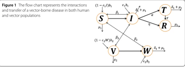
Figure 1The flow chart represents the interactions and transfer of a vector-borne disease in both human and vector populations
differential equations:
dS
dt = (1 –1I)b1–β1SI–β2SW–μ1S, dI
dt =1b1I+β1SI+β2SW–αI–ηI–δ1I–μ1I, dT
dt =αI–γT–δ1T–μ1T, dR
dt =ηI+γT–μ1R, dV
dt = (1 –2W)b2–β3VI–μ2V, dW
dt =2b2W+β3VI–δ2W–μ2W,
(1)
with the initial conditions
S(0)≥0, I(0)≥0, T(0)≥0, R(0)≥0, V(0)≥0, W(0)≥0. (2) The human host population is recruited at a constant birth rateb1in which a fraction1
were born infected from their infected parents.β1is the rate of direct transmission of the
disease,β2is the vector mediated transmission rate,μ1is the natural mortality rate of a
human. Infectious humans are treated at a rateα, recover naturally at a rateη, and suf-fer disease-induced death at a rateδ1. Treated humans recover at a rateγ. It is assumed
that recovered individuals acquire lifelong immunity against re-infection. Similarly,b3is
the constant recruitment rate of vector population in which the ratio2are infected by
birth from their infected parents. Susceptible mosquitoes become infected by biting in-fected human at a rateβ3,μ2is the natural mortality rate of vector population. Infectious
vectors die due to disease at a rateδ2. The complete dynamics of the proposed model is
represented by the flow chart in Figure 1.
2.1 Properties of solutions
Theorem 2.1 There exists a unique and bounded solution of the system of equations(1),
in a positively invariant set,that remains for all finite time t≥0.
Proof The right-hand side of each equation is continuous in the convex domain E= (t,S(t),I(t),T(t),R(t),V(t),W(t)) of (6 + 1)-dimensional spaceR6+1
+ with continuous partial
derivatives. So problem (1) has a unique solution inR6
+which exists for a given finite time t∈[0,∞) and initial conditions (2).
region for system (1) is
=
Thus the total populations and each population class remain bounded for all finite time
t≥0.
The above theorem shows that model (1) is well posed epidemiologically and mathemat-ically in a positively invariant set. We shall study the dynamics of this basic model in, so, all the solutions of system (1) start and remain infor allt≥0. All the parameters and state variables for the model should be non-negative for all time because they represent the number of the population sizes of humans and vectors.
3 Equilibrium points
3.1 Disease-free equilibrium
mean that the total recruited population is only susceptible. By direct calculations, we get the disease-free equilibrium pointE1in the feasible region, which is given by
E1= (S1,I1,T1,R1,V1,W1) =
The dynamics of model (1) is analyzed by a dimensionless number called basic repro-duction number denoted by R0, defined as “The expected number of secondary cases
produced by a typical infected individual during its entire period of infectiousness in a completely susceptible population” [31]. Mathematically,R0is defined as
R0∝
whereTis the transmissibility (i.e., probability of infection given contact between a sus-ceptible individual and an infected one),Cis the average rate of contact between suscepti-ble and infected individuals, andDis the duration of infectiousness. This quantity serves as a threshold parameter that predicts whether a disease will spread in a community or will simply die out. It can be calculated by the method of next generation matrix given in [32]. In the vector–host model (1), infected states areI,T, andW and uninfected states areS,R, andV. The matricesF andVare the rate of production of new infections and the transition rates between states, respectively, which are given by
F=
bian matrices at the disease-free equilibrium ofFandVareFandV, respectively, where
F=
FandV are the rates for new infections and transitions near the equilibrium. We used MATLAB(R2010A) to findV–1 andFV–1, which gives the times spent in each state and
largest eigenvalue ofFV–1is the basic reproduction numberR
0, given by
R0=
1b1+β1N1
k +
β2β3N1N2 mk ,
wherek=α+δ1+μ1+ηandm=δ2+μ2–2b2. When there is no vertical transmission,
1=2= 0, thenR0is the basic reproductive number for the model with only horizontal
transmission. Geometrically it means that the number of new infections comes from both direct and indirect transmission. In the presence of vertical transmission,1,2> 0,R0
in-creases as these vertical transmission parameters increase, because vertical transmission directly increases the number of infectious populations. Also we can see the inverse rela-tion of treatment strategies withR0and the direct relation with new infections and total
population.
The basic reproduction numberR0has a significant effect on the dynamics of infection.
As we can see from the first and second equations of model (1),
dS
dt =b1–kR0I–μ1S, dI
dt=k(R0– 1)I. (5)
WhenR0< 1, it means that each infected individual infects less than one other
individ-ual averagely by ever kind of transmission, then the change in the number of infected population is negative, so the disease simply dies out. On the other hand, whenR0> 1,
it means that each infected individual infects more than one other individual, then the change is positive and invasion is always possible (see the survey paper by Hethcote [33]). ForR0= 1, it means that each infectious individual infects one other individual as a whole,
then there is no change in the infected population, so the infection constantly remains in the population. Also the effect ofR0on the susceptible population is shown in the first
equation of (5). All these facts are shown in Figures 2 and 3.
Theorem 3.1 The disease-free equilibrium point E1is locally asymptotically stable if R0<
1,otherwise unstable.
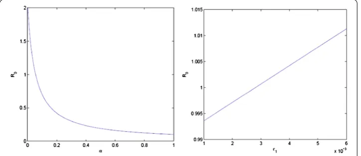
Figure 2The first figure shows thatR0decreases with increasing cure rate. The second figure shows thatR0
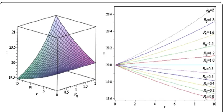
Figure 3The figures show the threshold behavior ofR0and its critical valueR0= 1
Proof This can be proved by linearizing system (1) aroundE1, which gives the following
Jacobian matrix:
J1=
⎡ ⎢ ⎢ ⎢ ⎢ ⎢ ⎢ ⎢ ⎢ ⎣
–μ1 –1b1–β1μ1b1 0 0 0 –β2
b1 μ1
0 1b1+β1μ1b1 –k 0 0 0 β2
b1 μ1
0 α –l 0 0 0 0 η γ –μ1 0 0
0 –β3μb22 0 0 –μ2 –2b2
0 β3μb22 0 0 0 –m
⎤ ⎥ ⎥ ⎥ ⎥ ⎥ ⎥ ⎥ ⎥ ⎦
,
wherel=γ +δ1+μ1.
The characteristic equation ofJ1is
(x+μ1)(x+μ1)(x+μ2)(x+l)
c0x2+c1x+c2
= 0, (6)
where
c0=μ1μ2,
c1=kμ1μ2+mμ1μ2–β1b1μ2–b11μ1μ2, c2=kmμ1μ2(1 –R0).
Four eigenvalues –μ1, –μ1, –μ2, and –lout of six have a negative real part. The remaining
two eigenvalues are the roots of the equationc0x2+c1x+c2= 0. ForR0< 1 andk+m>
β1N1+b11, we havec1> 0 andc1c2> 0. So, according to the Routh–Hurwitz criteria [34],
these two eigenvalues have a negative real part.
Since each eigenvalue of the characteristic equation (6) has a negative real part when
R0< 1, according to the Routh–Hurwitz method [34], system (1) is locally asymptotically
stable at the disease-free equilibrium pointE2and unstable whenR0> 1. The dynamical
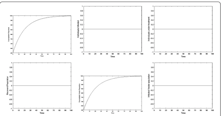
Figure 4The plots show the dynamical behavior of the model at disease-free equilibrium
3.2 Endemic equilibrium
The constant presence of a disease or an infectious agent within a given geographic area is called endemic. The endemic equilibrium state is the state where the disease cannot be totally eradicated but remains in the population. In order to find positive solutions of system (1), letE2= (S2,I2,T2,R2,V2,W2) represent any arbitrary endemic equilibrium.
Setting left-hand side equal to zero and solving the equations simultaneously at steady state, we obtain
Theorem 3.2 The endemic equilibrium point E2is locally asymptotically stable if R0> 1, otherwise unstable.
Proof To show these results, we linearize system (1) aroundE2, which gives the following
Two of the eigenvalues are –μ1and –l. The remaining eigenvalues are the eigenvalues of
We make an elementary row operation for the Jacobian matrixJ2∗to obtain the following matrix:
J2∗ is a lower triangular matrix and its eigenvalues are the elements of the main diagonal which are given by –Q, μ1QT –K, –μ2, and –M. Three of the eigenvalues have a negative
real part. The second eigenvalueμ1QT–Khas a negative real part if and only ifμ1QT–K< 0. Using the value ofQandT, we can rewrite this equation by rearranging it as follows:
–2β1β3K(δ2+μ2)I22+
β3(δ2+μ2)μ1K(1 –R0)
I2+μ2mμ1K(1 –R0). (7)
All the coefficients of this equation are negative ifR0> 1. Thus all the eigenvalues have
negative real parts, which shows that the endemic equilibrium pointE2is locally
asymp-totically stable iffR0> 1.
4 Global stability analysis
In this section, we study the global analysis of the disease-free and endemic equilibria using the direct Lyapunov method which requires the construction of a function with specific properties. In order to do this, we derive the following results.
Theorem 4.1 When R0< 1,then the disease-free equilibrium E1of system(1)is globally asymptotically stable on.
Proof To show the global stability of the disease-free equilibriumE1, we construct the
following Lyapunov function, following the method used in [35]:
ThenUisC1on the interior of,E
1is the global minimum ofUon, andU(t) = 0 at E1. Putting the values from model (1), we obtain
U(t) =1b1I+β1SI+β2SW–αI–ηI–δ1I–μ1I
{Ef}. Therefore, from LaSalle’s principle [36], the disease-free equilibriumEf is globally
asymptotically stable in.
Theorem 4.2 For R0> 1,the endemic equilibrium E2is globally asymptotically stable. Proof For the global stability of the endemic equilibria, we construct the following Lya-punov function:
Taking the time derivative of W, we get
Y(t) = 1
Rearranging equation (11), we get
Since
S S2
+S2
S ≥2 and V V2
+V2
V ≥2, (14)
because the arithmetic mean is greater than or equal to the geometric mean. ThusY(t)≤ 0 for all (S,I,T,R,V,W)∈and the equality (Y(t) = 0) holds forE2. The proof is
com-pleted as in the proof of Theorem (4.1).
5 Numerical simulation and graphs
We collect data from different sources and use the Runge–Kutta fourth order scheme to solve the model. Some of the parameter values are based on reality, for example, the death rate of humans by nature, corresponding to life expectancy of a 70-year-old human, is
μ1= 0.000039 per day, and the death rate of mosquitoes isμ2= 0.1 per day corresponding
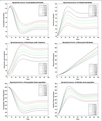
Figure 6The plots show the dynamical behavior of population sizes with increasing vertical transmission rate
to mosquito’s average life span of 10 days. Some of the parameter values are chosen from [25, 35]. The human’s and vector’s recruitment rates are b1= 20 and b2= 100 per day,
respectively. The disease-induced death rates of humans and mosquitoes areδ1= 0.01 and
δ2= 0.21, respectively.β1= 0.00001 andβ2= 0.0012 are the transmission probabilities of
dengue from human to human and vector to human population, respectively,β3= 0.001 is
the transmission probability of dengue from human to vector population. Given different values to the treatment parameter 0≤α≤1 to check the treatment effects. The natural recovery rate isη= 0.01, and the recovery rate due to treatment isγ= 0.4. We suppose the values of1,2and the initial population sizes. In rare cases the new offspring of infected
parents are infected so take1= 0.001 and the vertical transmission rate for mosquitos
is2= 0.002. For initial values, letS(0) = 100,I(0) = 30,T(0) = 25,R(0) = 10,V(0) = 600,
Figure 7The plots show the phase portrait of the susceptible human population versus the infected human population
Figure 8The plots show the phase portrait of the susceptible vector population versus the infected vector population
phase portraits of susceptible population versus infected population of human and vector populations, respectively.
6 Conclusion
The spread of different infectious diseases causes very high mortality rates in a popu-lation. Vector-borne diseases are infectious diseases transmitted to humans and animals through vectors. These diseases propagate from the infected to the susceptible population in different ways. This paper formulated an epidemic model for the transmission dynamics of vector-borne diseases with both vertical and horizontal transmissions with treatment strategy. The equilibrium points and the basic reproduction of the model are found. The basic reproduction number, which is a threshold quantity, has an important role in the epidemiology of the disease. As this number increases the disease invades the population, and as it decreases the disease simply dies out. Figure 2 shows thatR0decreases as
treat-ment strategies increase and increases as vertical transmission increases. Figure 3 shows the threshold behavior ofR0 and the critical valueR0= 1. AsR0increases, the infected
population increases with time. ForR0< 1, the number of infected population decreases;
forR0= 1, the infected population remains constant; and forR0> 1, the number of infected
lo-cally and globally asymptotilo-cally stable; and forR0> 1, the positive endemic equilibrium
is locally and globally asymptotically stable.
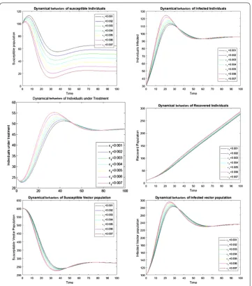
Numerical simulations are carried out graphically to show the dynamical behavior of the diseases. Figure 5 shows the effect of cure rate on the transmission dynamics of the disease. As treatment strategy increases, the susceptible population and the recovered human population increase while the infected population decreases. Figure 6 shows the effect of vertical transmission. As vertical transmission increases, the susceptible popu-lation decreases and the infected popupopu-lation increases. Finally, Figures 7 and 8 show the phase portraits of the susceptible populations versus the infected populations which move towards the stable points.
Acknowledgements
This work was supported by NNSFC (Grants 11571140, 11671077), Fellowship of Outstanding Young Scholars of Jiangsu Province (BK20160063), the Six Big Talent Peaks Project in Jiangsu Province (XYDXX-015), and NSF of Jiangsu Province (BK20150478).
Competing interests
The authors declare that they have no competing interests.
Authors’ contributions
All authors read and approved the final manuscript.
Author details
1Department of Mathematics, Faculty of Science, Jiangsu University, Zhenjiang, P.R. China.2Mathematics Department,
Faculty of Science, Taibah University, Al-Madinah Al-Munawarah, Saudi Arabia.3Mathematics Department, Faculty of Science, Beni-Suef University, Beni-Suef, Egypt.
Publisher’s Note
Springer Nature remains neutral with regard to jurisdictional claims in published maps and institutional affiliations.
Received: 29 November 2017 Accepted: 6 February 2018 References
1. Service, M.W.: Blood-Sucking Insects: Vector of Disease. Arnold, Victoriya (1986)
2. Wiwanitkit, V.: Unusual mode of transmission of dengue. J. Infect. Dev. Ctries.30, 51–54 (2009)
3. Antonis, A.F.G., Kortekaas, J., Kant, J., Vloet, R.P.M., Vogel-Brink, A., Stockhofe, N., Moormann, R.J.M.: Vertical transmission of rift valley fever virus without detectable maternal viremia. Vector-Borne Zoonotic Dis.13, 601–607 (2013) 4. Turchetti, A.P., Souza, T.D., Paix˘ao, T.A., Santos, R.L.: Sexual and vertical transmission of visceral leishmaniasis. J. Infect.
Dev. Ctries.8(4), 403–407 (2014)
5. Buckner, E.A., Alto, B.W., Lounibos, L.P.: Vertical transmission of Key West Dengue-1 virus by Aedes aegypti and Aedes albopictus (Diptera: Culicidae) mosquitoes from Florida. J. Med. Entomol.50(6), 1291–1297 (2013)
6. The World Health Report 2014: Changing history, WHO, Geneva, Switzerland
7. World Health Organization: Dengue and dengue haemorrhagic fever, Geneva, Report (2002)
8. Yang, X.J., Gao, F.: A new technology for solving diffusion and heat equations. Therm. Sci.21, 133–140 (2017) 9. Yang, X.J.: A new integral transform with an application in heat-transfer problem. Therm. Sci.20, S677–S681 (2016) 10. Abdullah, Seadawy, A.R., Jun, W.: Mathematical methods and solitary wave solutions of three-dimensional
Zakharov–Kuznetsov–Burgers equation in dusty plasma and its applications. Results Phys.7, 4269–4277 (2017) 11. Yang, X.J.: A new integral transform operator for solving the heat-diffusion problem. Appl. Math. Lett.64, 193–197
(2017)
12. Yang, X.J.: New integral transforms for solving a steady heat transfer problem. Therm. Sci.21(1), S79–S87 (2017) 13. Seadawy, A.R.: Two-dimensional interaction of a shear flow with a free surface in a stratified fluid and its solitary-wave
solutions via mathematical methods. Eur. Phys. J. Plus132, 518 (2017)
14. Lu, D., Seadawy, A.R., Arshad, M.: Bright–dark solitary wave and elliptic function solutions of unstable nonlinear Schrödinger equation and their applications. Opt. Quantum Electron.50, 23 (2018)
15. Kumar, D., Seadawy, A.R., Joardar, A.K.: Modified Kudryashov method via new exact solutions for some conformable fractional differential equations arising in mathematical biology. Chin. J. Phys.56, 75–85 (2018)
16. Seadawy, A.R., El-Rashidy, K.: Traveling wave solutions for some coupled nonlinear evolution equations. Math. Comput. Model.57, 1371–1379 (2013)
17. Seadawy, A.R.: Stability analysis solutions for nonlinear three-dimensional modified Korteweg–de Vries–Zakharov–Kuznetsov equation in a magnetized electron-positron plasma. Physica A455, 44–51 (2016) 18. Lu, D., Seadawy, A.R., Arshad, M.: Applications of extended simple equation method on unstable nonlinear
Schrödinger equations. Optik140, 136–144 (2017)
20. Seadawy, A.R.: The generalized nonlinear higher order of KdV equations from the higher order nonlinear Schrödinger equation and its solutions. Optik139, 31–43 (2017)
21. Seadawy, A.R.: Three-dimensional nonlinear modified Zakharov–Kuznetsov equation of ion-acoustic waves in a magnetized plasma. Comput. Math. Appl.71, 201–212 (2016)
22. Blayneh, K.W., Jang, S.R.: A discrete SIS-model for a vector-transmitted disease. Appl. Anal.85, 1271–1284 (2006) 23. Bowman, C., Gumel, A.B., Driessche, P.V.D., Wu, J., Zhu, H.: A mathematical model for assessing control strategies
against West Nile virus. Bull. Math. Biol.67, 1107–1133 (2005)
24. Ali, N., Zaman, G., Abdullah, Alqahtani, A.M., Alshomrani, A.S.: The effects of time lag and cure rate on the global dynamics of HIV-1 model. BioMed Res. Int.2017, Article ID 8094947 (2017)
25. Lashari, A.A., Zaman, G.: Global dynamics of vector borne disease with horizontal transmission in host population. Comput. Math. Appl.61, 745–754 (2011)
26. Khan, T., Zamana, G., Chohan, M.I.: The transmission dynamic and optimal control of acute and chronic hepatitis B. J. Biol. Dyn.11, 172–189 (2016)
27. Khan, T., Jung, I.H., Khan, A., Zaman, G.: Classification and sensitivity analysis of the transmission dynamic of hepatitis B, pp. 14–22 (2017)
28. Ross, R.: The Prevention of Malaria, 2nd edn. Murray, London (1911)
29. Macdonald, G.: The analysis of equilibrium in malaria. Trop. Dis. Bull.49, 813–828 (1952)
30. Lashari, A.A., Hattaf, K., Zaman, G., Li, X.-Z.: Backward bifurcation and optimal control of a vector borne disease. Appl. Math. Inf. Sci.7, 301–309 (2013)
31. Diekmann, O., Heesterbeek, J.A.P., Metz, J.A.J.: On the definition and the computation of the basic reproduction ratio R0in models for infectious diseases in heterogeneous populations. J. Math. Biol.28, 365 (1990)
32. Driessche, P.V.D., Watmough, J.: Reproduction number and sub-threshold endemic equilibria for compartmental models of disease transmission. Math. Biosci.180, 29–48 (2002)
33. Hethcote, H.W.: The mathematics of infectious diseases. SIAM Rev.42, 599 (2000)
34. Rao, V.S.H., Rao, P.R.S.: Dynamic Models and Control of Biological Systems. Springer, Dordrecht (2009) 35. Garbab, S.M., Safi, M.A., Gumel, A.B.: Cross-immunity-induced backward bifurcation for a model of transmission