R E S E A R C H
Open Access
Cognitive radio engine parametric optimization
utilizing Taguchi analysis
Ashwin E Amanna
*, Daniel Ali, Manik Gadhiok, Matthew Price and Jeffrey H Reed
Abstract
Cognitive radio (CR) engines often contain multiple system parameters that require careful tuning to obtain favorable overall performance. This aspect is a crucial element in the design cycle yet is often addressed with ad hoc methods. Efficient methodologies are required in order to make the best use of limited manpower, resources, and time. Statistical methods for approaching parameter tuning exist that provide formalized processes to avoid inefficient ad hoc methods. These methods also apply toward overall system performance testing. This article explores the use of the Taguchi method and orthogonal testing arrays as a tool for identifying favorable genetic algorithm (GA) parameter settings utilized within a hybrid case base reasoning/genetic algorithm CR engine realized in simulation. This method utilizes a small number of test cases compared to traditional design of experiments that rely on full factorial combinations of system parameters. Background on the Taguchi method, its drawbacks and limitations, past efforts in GA parameter tuning, and the use of GA within CR are overviewed. Multiple CR metrics are aggregated into a single figure-of-merit for quantification of performance. Desirability functions are utilized as a tool for identifying ideal settings from multiple responses. Kiviat graphs visualize overall CR performance. The Taguchi method analysis yields a predicted best combination of GA parameters from nine test cases. A confirmation experiment utilizing the predicted best settings is compared against the predicted mean, and desirability. Results show that the predicted performance falls within 1.5% of the confirmation experiment based on 9 test cases as opposed to the 81 test cases required for a full factorial design of experiments analysis.
Keywords:cognitive radio, cognitive engine, design of experiments, Taguchi method, parametric optimization
1 Introduction
Cognitive radios (CRs) incorporate artificial intelligence with wireless communications devices to enable automated decision making and long term learning. Architectures for cognitive engines (CE) include rules, meta-heuristics, and experientially based as well as hybrid combinations. Even rudimentary architectures generate several configuration parameters that require careful tuning to achieve favorable performance. Realistic constraints of time, manpower, and resources place limitations on the amount of testing avail-able to address this element of CR design and develop-ment. The same constraints apply to overall system testing of CR.
Trial and error approaches toward selecting CE para-meter values make poor use of available resources. The specific problem addressed here focuses on implementing
strategies that limit the number of required tests needed to identify acceptable parameter values. These same meth-odologies can be applied to overall system testing. The pri-mary goal centers on defining satisfactory ranges of performance rather than identifying computationally opti-mum values. Several systematic frameworks exist that address this problem from a statistical perspective utilizing empirically measured results. These methods include design of experiments (DOE), response surface methodol-ogy (RSM), and the Taguchi method utilizing orthogonal arrays (OA). These methods are well accepted across many fields of science and production environments [1,2]. However, as the number of configuration variables grows, the benefits of DOE and RSM formalizations diminish due to the significant number of test cases that full factorial designs require. DOE requires testing of all the maximum and minimum values of each combination of parameters, while RSM requires the addition of nominal values. For example, a four-variable configuration with three levels
* Correspondence: [email protected]
Bradley Department of Electrical and Computer Engineering, Wireless @ Virginia Tech, Blacksburg, VA, USA
each requires 34= 81 individual test cases. Each test case will require at least two runs to determine variance, increasing the minimum required runs to 162. These trade offs between test case quantities and value-added informa-tion gained will be an important issue as CR matures to field deployments.
This article explores the use of the Taguchi method to identify selection of genetic algorithm (GA) configuration parameters within a CR engine. The Taguchi method uti-lizes an efficient selection of testing configurations based on the concept of OA. Experimenters have utilized OAs since the 1940s; these are based on statistical designs that yield sufficient knowledge to determine a favorable para-meter setting with a limited number of experimental runs [3]. The Taguchi method is implemented on the GA mod-ule within a CE designed around a railway application for transmission of packet data [4]. This CE utilizes a hybrid architecture of case-based reasoning (CBR) decision mak-ing with GA-based optimization. The figure-of-merit (FOM) concept, used in performance analysis of computer network systems [5], defines a quantification of perfor-mance that is an aggregate of several CR metrics as opposed to only the fitness function used within the GA calculations.
This article differs from others that focus on GA para-meter optimization by measuring GA performance within the context of an overall CE. The fitness function utilized within the GA is one of several performance metrics that are aggregated for analyzing the data within the Taguchi method framework. While DOE methodologies have been applied within the context of CR [6], to the best of our knowledge, Taguchi methods have not. The methodology presented contributes a systematic framework that can be applied across other components of CEs regardless of the specific application spaces. Additional unique aspects include the use of aggregate FOM for quantification of performance, the use of Kiviat graphs as a visualization of CE behavior, and formulation of Taguchi methods within a CR application.
The remainder of this article is structured as follows. Section 2 provides background on the use of GAs within CR and efforts for identifying ranges for parameter set-tings. An overview of the Taguchi method is provided as well as drawbacks and limitations of the method compared to other statistical methods such as DOE and RSM. Sec-tion 3 describes the overall CE architecture and process flow between the experientially based CBR and GA. Per-formance metrics and FOM are described. Section 4 defines the experimental design of the system model and selection of the L9 OA utilized within the Taguchi method. Section 5 discusses the results from running each test case of the OA on the system and the results of the analysis which lead to a predicted best parameter setting. A confirmation experiment is run using the predicted best
parameter settings and compared against the calculated performance. Finally, Section 6 summarizes and suggests areas for further research.
2 Background
This section briefly reviews the GA, past use of the GA in CRs, and efforts to identify parameter settings. One can follow the testing methodology presented here without intimate knowledge of the GA due to the viewpoint that systems being tested can be considered as‘black boxes’ where input parameters are defined and performance measures observed. Results are presented only in terms of the input configuration parameters. This concept is important from the perspective of system development and deployment, where only a few key individuals may possess detailed knowledge of how components are designed, and others will most likely test and configure the system. This section also reviews the basics of the Taguchi method, OA, and desirability functions as evalua-tion tools for Taguchi analysis.
2.1 GA background
This section provides a cursory review of the operation of a GA. A more detailed review can be found in [7]. Evolu-tionary processes provided the inspiration for the GA as a tool for optimization of a function. Biological cells are defined by strings of DNA known as a chromosome. Each chromosome contains a set of genes comprised of blocks of DNA. These genes define physical attributes of the cell or organism, such as hair color. As organisms reproduce, the genetic information from both parents is combined into new chromosomes comprised of genes from both parents. In addition, random mutations occur that change individual genes. A measure of success of an organism is its fitness, or how much it can reproduce before it dies. The concept of‘survival of the fittest’states that the best combination of genes and their resulting chromosomes yields the strongestindividualwhich will survive the longest.
utility function is then combined into a single fitness value.
The GA starts by creating apopulationof several indivi-duals. Each individual’s fitness is assessed, and individuals are ranked in order of highest fitness. Top individuals becomeparentsfor the next generation of the GA, while the weakest performers are discarded. Thechildrenof sur-viving parents are created by crossing over genes between parents. In this manner, strong characteristics from two sets of parents are combined as shown in Figure 1. In addition, random mutations of single bits within a chro-mosome are implemented based on a probability density function enable searching more of the variable space.
2.1.1 GA use in CR
CR architectures have gravitated towards GA as potential decision-making algorithms given their capability of sol-ving complex spaces based on multiobjective definitions [8]. Performance in CR must be defined in terms of multi-ple elements, such as bit error rate (BER), bandwidth, throughput, and transmit power. Utilization of GA within wireless communications application space required mod-eling the physical (PHY) layer traits of the radio within the context of a genetic chromosome. PHY layer characteris-tics such as BER, modulation, and frequency were repre-sented as variable bit representations of genes. Nonlinear utility functions were utilized to convert PHY layer meters into values between [0,1]. These utilities were aggregated into weighed fitness functions that could be tuned to emphasize specific radio missions such as minimizing transmit power or maximizing throughput [9]. These initial groundbreaking works spawned many research directions that range from sensitivity analysis [10] of the individual elements of the chromosomes to the incorpora-tion of other bio-inspired algorithms.
A typical process flow for the use of a GA within CR is as follows:
1. The radio parameters each represent a gene which are encoded together to form a chromosome.
2. The initial population is created either from ran-dom generation, or from the output of other modules of a cognitive engine, such as a case based reasoner [4].
3. During each generation, the chromosome’s genes
are decoded to identify the suggested radio parameters. 4. The radio parameters are used to estimate perfor-mance meters. Both the parameters and estimated meters are normalized using utility functions and com-bined into a single measure of fitness.
5. The next generation is created by crossing over genes from the parents with the highest fitness.
6. Each bit of the population is randomly mutated with a fixed probability.
7. The algorithm repeats the process for a defined number of generations.
While powerful, the heuristic nature of the algorithm was plagued with slow operations. To enhance decision making speed, the GA architecture was hybridized with experientially based decision making such as CBR. Experiential databases provide a faster first attempt to match the current situation with a successful decision made in the past. If a sufficiently similar case is not found, the top retrieved cases can act as partial seeds into a GA with the goal of improving performance [11]. This architecture is utilized within this article and will be discussed in more detail in Section 3.
2.1.2 Identifying GA parameters
The selection of GA configuration parameters will have bearing on the success of the algorithm. The key para-meters are crossover rate, mutation rate, population size, and maximum generations.
1.The crossover rate, or probability of crossover, affects the rate at which crossover between parents occur. A higher crossover rate, increases new strings into the population faster. Too low a crossover rate will limit the exploration rate due to lower number of potential solu-tions. Mutation rate is the probability that each bit of the string undergoes a random flip after the selection of a new parent.
2. Mutation rates affect the speed of searching. Too high a rate makes the search similar to a random search which can be inefficient. Too low a rate limits the diver-sity of the population making finding the best solution harder.
3. Population size controls the amount of chromo-somes that the GA has in each generation. Too big a population size requires a longer search of the current generation to identify the best ones of the generation which will become the parents of the next generation. However, too small a population again limits future diversity.
4.Maximum generationslimits the number of iterations that the GA is allowed to make before a final solution is identified. GA’s are known to converge to near-optimal solutions, however the time it takes to reach a solution is an important consideration. In CR, the environment may change before the GA has had a chance to fully converge, therefore maximum generations cannot be too high. This leads to having to make some concessions into the final fitness of the solution. It may not have converged on the overall best solution. In this case, a‘good-enough’solution maybe a necessity.
Since the inception of GA, there have been several efforts to identify ideal parameter settings. De Jong’s key work evaluated four parameters: population size, cross-over rate, mutation rate, and generation gap [12]. His conclusions provided recommended ranges that are con-sidered default settings for basic GAs. The suggested guidelines were population size: 50-100; crossover rate: 0.6; and mutation rate: 0.001. Work by Schaffer et al. [13] investigated interaction effects between parameter settings and suggested an inverse relationship between population size and mutation rate. This effort led to recommendations for parameter ranges of population size: 20-30; mutation rate: 0.005-0.1; and crossover rate: 0.75-0.95. The Taguchi method has been applied to the problem of identifying GA parameters using the same theoretical test objective functions as utilized by DeJong [14]. The results indicated that GA parameter settings were dependent on the specific test application.
With regard to interaction effects between parameters, Rezende performed statistical analysis utilizing the DOE methodology to identify these relationships between popu-lation size, number of generations, crossover probability, and mutation probability, as well as the qualitative factors of crossover type and mutation type [15]. Results indicated that crossover type had the most effect on performance, and interaction effects were most prevalent between popu-lation size, maximum number of generations, crossover rate and type of crossover, and mutation rate and type of crossover. The statistical value of the interaction effect between population size and maximum number of genera-tions was 0.03 wherep= 0.05 is the typical cutoff. There-fore, this interaction is considered relatively weak.
2.2 Taguchi method
The Taguchi methods were developed as an alternative to traditional DOE which have been in use since the early
1930s [16]. This section will review the Taguchi method of experimental design. First, the efficient OA representation of test cases is presented, followed by the concepts of Tagu-chi signal to noise ratio. A top level process flow for the Taguchi method starts with selecting parameters and their levels, running a number of individual test cases containing a unique combination of these parameters, measuring the output, and calculating output means and variations.
DOE methods study the effects of the variation of input parameters on a system or process. Fundamentally, the system or process is viewed as a black box such that input parameters are implemented and output perfor-mance measures are tracked. Rather than changing only one variable at a time, multiple variables are changed between experimental runs in order to isolate interaction effects between control parameters. Each parameter is represented as a range of potential values. In a full factor-ial design, each potentfactor-ial combination of parameter values is tested. As the number of parameters grows, the number of tests required can quickly expand beyond the realistic capabilities of the testers.
Taguchi differed from traditional DOE in a number of ways. First, a more efficient array of test conditions was developed that significantly decreased the number of test cases required in order to draw performance conclusions. Consider a system withPconfiguration parameters andL
levels, and test plans withNtotal test cases. A traditional full factorial design requiresN=LPunique configura-tions to test each combination of parameters and levels.
Consider a system withP = 10 andL = 3. This would
require 310= 59, 049 test cases for a full factorial design. The number of runs can essentially be considered a cost. An OA has potential for similar information gain about the system at a much lower cost. Taguchi recognized the need for reduced testing matrices given the realistic con-straints on time, manpower, and resources. His perspec-tive was from the manufacturing perspecperspec-tive where these constraints are very prevalent; therefore, his methods centered on OA concepts developed in the 1940s [17].
Orthogonal array design
This section describes the OA testing matrix that provides an efficient combination of configuration parameters to minimize the resource cost from testing. The notation for this array is defined asOA(N,k,s,t) where an array,Aof size N×kis created fromkparameters consisting of s
levels which are a subset ofSand strengthtsuch that (0≤
t≤ k) [18]. The selection of strength is driven by the potential for interaction amongst factors. Pairwise interac-tion between any two parameters is adequately address with a strength oft= 2. One can increasetto incorporate higher order interactions, at the cost of more tests. Strength of 2 is adequate for this application.
are rows for every N × t sub-array of the overall A
matrix. Weng et al. [19] provide an example of anOA
(27,10,3,2) utilized in the design of a linear antenna array based on the Taguchi method. Here we utilize an
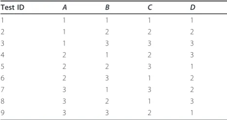
OA(9,4,3,2) which is also known as the L9 array as
shown in Table 1. The“L”is related to the classic Latin Square design which OAs are based upon. The elements of the array are selected fromS = 1, 2, 3 representing three discrete levels of the GA control parameters which are mapped to the labels:A,B,C, D.
Following the illustrative example of [19], any two col-umns, as defined byt= 2 will always show nine possible combinations in the rows: (1,1), (1,2), (1,3), (2,1), (2,2), (2,3), (3,1), (3,2), and (3,3). These combinations appear as many times as there are rows. In this case, they appear nine times. Each row represents a unique test case where the control parameters are set to the designated level. For example, test ID 7 of the OA(9,4,3,2) sets parameter A to level 3, parameter B to level 1, C to level 3, and D to level 2. This array type is also known as a fractional factorial representation of a full factorial array which would have 81, or 34unique test cases. Given the small number of test cases compared to full factorial designs, it is common that the resulting best case after the analysis was not among the cases within the OA. Therefore, it is common to run a
confirmation experimenton the resulting case.
Taguchi methods are also known for their capability to investigate the response output created from combinations of controllable parameters and uncontrollable parameters. The OAs described above are also known as inner arrays. A second array can also be incorporated around each point of the inner array that includes variations of uncontrollable parameters. For the purposes of testing, these typically uncontrollable parameters are fixed at mini-mum and maximini-mum values of their uncontrollable para-meters’range. This is often called the outer array. This article only considers inner array test cases.
2.2.1 Taguchi signal-to-noise ratio
Another key area in which Taguchi differs from traditional DOE methods focuses on the success of the output. Tradi-tional methods strive to identify and maximize/minimize
the mean output of a system. Taguchi’s production back-ground trained him to emphasize not only mean output but also to minimize the variation around that target which is a truer measure of overall quality. Taguchi refers to this relationship between variation and the output as signal-to-noise ratio (SNR). To avoid confusion with com-mon wireless communications terminology, this article will refer to this as SNRTag. There are three distinct
for-mulas for calculation of SNRTag: (1) lower-is-better (LIB)
as shown in 1; (2) higher-is-better (HIB) as shown in 2; and (3) nominal-is-better (NIB) as shown in 3 [20]. Each sample of the metric under consideration is denoted asyi
andyis the overall sample mean given fromnreplicates. The variance in of the sample is denoted ass2. In other
words, the LIB SNRTag is -10log[mean of the sum of
squares of measured data], and the HIBSNRTagis -10log
[mean of sum of squares of reciprocal of measured data],
and the NIBSNRTagis -10log[square of the
mean/var-iance].
Analysis of Taguchi designs proceeds by testing each case within the OA. A desired target or the overall goal of HIB or LIB must be identified. The output response is measured as a result of each test case. Multiple runs are averaged, and the mean and SNRTag are calculated.
These values are further analyzed utilizing desirability functions and discussed in more detail in Section 5.
2.3 Drawbacks and limitations
There are several drawbacks and limitations when follow-ing the basic Taguchi methodology. First, each parameter value requires discrete values. Predicted results are only calculated at these discrete values. In contrast, the RSM methodology enables prediction at points not located at dedicated values of the control parameters. Second, the method discussed assumes that interaction effects between parameters are negligible. A complete DOE screening that evaluates every combination of parameter values has the capability of identifying interaction effects amongst parameters. In many cases this is not feasible given the sheer quantity of test cases required. Often, experimenter knowledge of the overall systems enables intuitive judgments about which effects lend themselves towards interaction.
Table 1 OA(9,4,3,2) L9 orthogonal array
The Taguchi method predicts a parameter setting that will result in the best performance based on the initial definition. It is unable to define a model for the system behavior. RSM techniques are suggested for this level of system understanding; however, the cost in terms of increased testing cases can be significant. The analysis pro-cess for identifying a favorable parameter set is performed offline and typically is not conducive to an automated pro-cess for real-time operations. Therefore, the Taguchi method alone might not provide a real-time solution for CE operations. There are several hybrids of the Taguchi method with heuristic methods, such as a GA, which might provide more real-time functionality [21]. Finally, the resulting solution set of configuration parameters typi-cally requires a confirmation test in which these para-meters are run through the testing configuration.
3 CE architecture
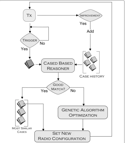
This section overviews the CE architecture utilized within this article. Figure 2 illustrates the process flow [22]. The CE is tethered to a software-defined radio such that it pulls system parameter information from the radio and pushes new configurations. The engine maps the config-uration parameters of the radio (commonly known as ‘knobs’) as well as radio performance metrics (commonly known as‘meters’) into a vector representation. This vec-tor enables the use of similarity calculation for CBR-based engines to compare different situations against each other. CBR is founded on the belief that solutions to new situa-tions can be identified based on solusitua-tions used in similar situations in the past. This is discussed in more detail in [22-24]. The decision process utilized in this article first attempts to utilize the CBR. If a past decision does not fall within a defined similarity threshold, then the CE calls the GA. Only GA configuration parameters are changed between test runs, as indicated in Table 1.
When a CE engine is initialized without a case base, it must rely on the GA to make decisions. Each time a favor-able decision is made such that performance improves after the decision, that case is added into the past history as a successful decision. CBR case retrieval is based on a combination of similarity to the current situation as well as the resulting success of the past decision. Therefore, past decisions that also have a high fitness have a better chance of being retrieved as a potential solution to a new situation. Ideally, this case can be retrieved in the event that a future situation matches this past situation.
This article does not take into consideration the inter-action effects between CBR configuration parameters and the GA operations as all CBR configuration variables are kept constant between test runs. In addition, the case-based history was erased between each run and between each test configuration. Typically, past history would remain in place across multiple runs. New successful
cases augment past history to provide the capability to learn from past experiences.
3.1 Utility and fitness definitions
There is a multi-step process for calculating the fitness function utilized within the GA module of the CE. First, knobs and meters are converted to a utility with values between [0,1]. This conversion is not a direct normaliza-tion, but rather makes use of dedicated utility functions to place the value on this scale. The utility functions presented in Equations (4)-(6) are based on previous work [11].
The fitness function utilized within the GA consists of a weighted sum of the above utility functions, as shown in (7). The weights are driven by user-designated radio missions, as discussed in [9]. These missions include minimize transmit power, maximize throughput, and minimize BER. This article utilizes the minimize-BER mission with weights set towTX = 0.0725, wBER = 0.8,
andwThroughput= 0.0725.
f =
i
wiui (7)
3.2 Estimation methods within the GA
The GA must estimate performance metrics of the members of the population in order to calculate the fit-ness of each individual. The reliance on estimations is one drawback of the GA. The performance parameters estimated include the radio SNR, throughput, BER, and packet error rate (PER), and spectral efficiency.
The estimation methodologies are adapted from [8,25]. The estimations assume an Additive White Gaus-sian noise (AWGN) channel. It is acknowledged that this is a simplified model that does not take into account fading, or interference. It does however, provide a benchmark environment for characterizing how Tagu-chi designs perform on a basic wireless system.
3.3 Metrics
performance metrics are aggregated to produce a single quantification of performance. These metrics, as shown in Table 2, include BER, number of decisions made
using the GA, average fitness after a decision is made, average throughput, number of decisions made using CBR, and average time to action. The architecture will
operate with faster decision cycles the more that it can use the CBR over the GA, and operate with higher fit-ness performance if better decisions are made. There-fore, the GA parameter settings are judged with regard to improvements of fitness post-decision, how fast deci-sions are made, and how often the engine is able to rely on the CBR for decisions. These metrics can also be broadly categorized as HIB and LIB. BER can be viewed as a LIB metric in its standard form, or converted to HIB by dividing the BER by a target-goal BER. In this case, BER is converted to HIB. The use of the Merrill’s FOM is suggested to combine alternating HIB and LIB metrics into a single quantified value as shown in (8)
[5]. Where nis the number of metrics considered, and
xiis an individual metric. The metrics are ordered such
that when i is odd, the metric is HIB, and when i is
even the metric is LIB. The Resulting FOM is a single aggregate quantification of the multiple metrics on a normalized scale.
The FOM is not without its drawbacks. It considers all axes and metrics of equal weighting, and extreme values are viewed as favorable. This may not always be the case. Equal FOM values between two different systems do not mean that the systems are equally as good. There could be imbalances in the system which the FOM calculation does not show.
4 Experimental design
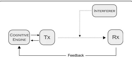
A transmit-receiver chain and external interference source realized in simulation comprised the system model, as shown in Figure 3. A data file was transmitted to the receiver utilizing BPSK modulation, forward error
correction coding, and additive white Gaussian noise injected into the system. The CE was required to make a decision regarding whether to change transmit power, or coding in response to changes in system perfor-mance. Feedback of received BER, presence of and mag-nitude of external interference power were assumed. A decision cycle consisted of (1) observation of received BER and interference power; (2) making a decision uti-lizing either the CBR or the GA to change or maintain existing settings of either the transmit power or coding; (3) observing the resultant performance metrics after a decision; and (4) augmenting the existing case-based history if a decision resulted in improved performance. After the tenth decision cycle, a simulated external interference source was engaged. The interference was turned off after the twentieth decision cycle and the test ended after 30 decision cycles. Each decision cycle pro-vided performance measures in terms of overall system fitness and time-to-action for each decision whether the CBR or the GA was utilized.
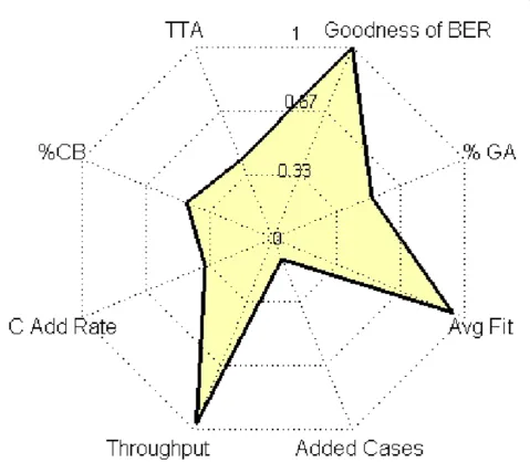
Figure 4 illustrates the results from one example test run. Thex-axis represents the decision index. Stars indi-cate that the GA was utilized to make the decision, while circles indicate that the CBR made the decision. Successful decision made by the GA are saved into the case base history for retrieval by the CBR based on simi-larity calculations. The resulting metrics across 30 deci-sion indexes are averaged and then combined into the FOM as defined by (8). This example resulted in a FOM = 0.7833 and is illustrated by the Kiviat graph shown in Figure 5. These charts are designed to quickly illustrate balanced performance where a symmetrical star shape is ideal.
Typically, a CE would operate in an event-driven cycle such that a decision process is entered only if predefined metrics go outside of defined specifications. In this test-ing protocol, the engine was operated in a forced deci-sion mode such that decideci-sions were required every cycle to generate a higher number of decisions per test. Even if the engine was selected to not make a change to exist-ing knob settexist-ings, this was still considered a decision.
Table 2 Metrics: the performance metrics used to quantify improvement or degradation are broadly categorized as either higher-is-better(HIB) or lower-is-better(LIB)
Average Time To Action LIB
BER was converted from a LIB to a HIB by considering the utility,or goodness o BER. This was done to balance the number of HIB and LIB which makes Kivia charts more readable.
The GA parameters manipulated between test runs were (A) crossover rate; (B) mutation rate; (C) popula-tion size; and (D) allowable maximum generapopula-tions. The ranges of values these parameters take were selected based upon findings discussed in Section 2.1.2. The values of each of these parameters were mapped into three discrete values, as shown in Table 3.
5 Results
Nine separate testing configurations of GA parameters were tested. Each configuration test was repeated five times. The overall FOM for each replicate of the test was
recorded as shown in Table 4. SAS JMP 9.0statistical
software package was utilized for the analysis of the Taguchi testing matrix. The SNRTagutilizing an HIB goal
per (2) was calculated for each test configuration along with a calculation of desirability on a scale of [0,1].
Desirability functions are a common tool for assessing optimization of multiple responses and are crafted to match the desired HIB or LIB goals [26]. Desirability functions are similar to the the utility functions dis-cussed in Section 3.1 in that the functions map the response variable to a [0,1] scale where 0 is least desir-able and 1 is most desirdesir-able. These mappings, defined as
di, take on different shapes depending on if the goal of
the overall response was identified as an HIB, LIB, or nominal. An overall desirability, defined asD, is com-prised of a geometric mean of each dias shown by (9).
In this form, all parameters are and their responses are
weighted equally. JMPdefined piecewise smooth
func-tions for desirability based on the default settings.
D= n
n
i=1
di (9)
The analysis package calculated a prediction profile for each parameter, as shown in Figure 6. These profiles illustrate the output response as a single element as var-ied while the other three are kept constant [27]. This figure also indicates the configuration settings that lead to a predicted best performance, as indicated by the red dotted lines. To read the chart, one identifies the para-meter of interest such as crossover rate. As crossover rate varies from value 1, 2, and 3, the output trend tends to increase. This assumes that the other three parameters are kept constant.
parameters is generated. The parameter configuration of [A = 3,B= 1,C = 2,D = 2] was identified as the pre-dicted best combination to achieve the desired output response.
5.1 Confirmation experiment
The predicted best testing configuration was not one of the original configurations of the L9 orthogonal matrix. Therefore, a confirmation experiment was run imple-menting the suggested configuration in order to verify performance. Table 5 shows the results of these tests Figure 5Kiviat graph: The Kiviat graph, also known as a spider chart graphically combines performance across multiple metrics in one figure. Similar to utilities that are normalized between [0,1], each metric is placed on the same scale. Higher-is-better, and lower-is-better metrics are alternated such that a balanced system is star shaped. The FOM is like fitness in that it is an aggregate combination of all metrics. The FOM of this example is 0.7833.
Table 3 GA testing parameter values
Parameter 1 2 3
A: crossover rate 0.55 0.675 0.95
B: mutation rate 0.005 0.0075 0.01
C: population size 50 75 100
D: maximum generations 25 50 75
and comparison to predicted performance. The confir-mation experiment indicated that resulting mean FOM
was 1.50% less than predicted, SNRTag was 14.52%
worse than predicted, and desirability was 4.58% less than predicted. Figure 7 shows the resulting Kiviat graph of one of the confirmation experiments for FOM = 0.8612.
6 Conclusions
This article presented an application of the Taguchi method that utilized orthogonal testing matrices for
optimizing configuration parameters of a GA utilized within a CR engine. Testing methodologies like these provide an efficient means for assessing performance without testing across the entire range of potential con-figurations. Results indicate that a nine fold decrease in the number of required experiments elicited a predicted configuration parameter set that fell within 1.50% of the actual FOM performance metric. While unsuitable for drawing conclusions on true optimality, these methods provide general trends of performance and provide a tradeoff between minimizing testing costs and
Figure 6Prediction profiler: The prediction profiler tool enables simple multi-objective near optimization of response factors based on defined goals. Profile traces are displayed where theX-axis is the factor and theY-axis is the output response. The profile trace is the predicted response as theX-axis variable changes while the other variables are held constant. The far right column are the defined desirability functions for each response. In this case both are set to a‘higher-is-better’shape. A recursive search function enables identification of theXvariables which lead to maximizing the total desirability.
Table 4 Collected data
ID A B C D run-1 run-2 run-3 run-4 run-5 mean SNRTag d
1 1 1 1 1 0.6488 0.6465 0.6504 0.6535 0.6613 0.6521 -3.7145 0.0762
2 1 2 2 2 0.7546 0.7574 0.7586 0.7590 0.7557 0.7571 -2.4175 0.5035
3 1 3 3 3 0.7284 0.7282 0.7308 0.7330 0.7285 0.7298 -2.7363 0.3922
4 2 1 2 3 0.8433 0.8436 0.8451 0.8483 0.8438 0.8448 -1.4648 0.8746
5 2 2 3 1 0.6700 0.6691 0.6760 0.6820 0.6753 0.6745 -3.4212 0.1690
6 2 3 1 2 0.8393 0.8180 0.8418 0.8428 0.8451 0.8374 -1.5432 0.8430
7 3 1 3 2 0.8603 0.8604 0.8606 0.8612 0.8630 0.8611 -1.2990 0.9423
8 3 2 1 3 0.7736 0.7750 0.7757 0.7749 0.7749 0.7748 -2.2160 0.5777
9 3 3 2 1 0.7346 0.7229 0.7753 0.7382 0.7423 0.7427 -2.5913 0.4432
knowledge gained on system performance. Further research suggested includes comparing this analysis to one utilizing RSM to develop an overall model of system performance and confirming the state of interaction
effects between parameters. In addition, this effort focused on a single module within the cognitive archi-tecture. A similar DOE that considers interaction and performance effects of varying configuration parameters
Table 5 Confirmation experiment results
ID A B C D run-1 run-2 run-3 run-4 run-5 mean SNRTag d
Predicted 3 1 2 2 0.8742 -1.1363 0.9865
Confirmation 3 1 2 2 0.8602 0.8619 0.8607 0.8604 0.8611 0.8609 -1.3014 0.9413
Difference (%) -1.50 -14.52 -4.58
The desirability analysis yields a recommended configuration that will maximize desirability. This configuration was not one of the designs within the L9 matrix. Only a predicted response and desirability is provided in the model. Therefore, the configuration was entered into the simulation and run in order to confirm the prediction. The means were recorded for each run. Results show a 1.5% difference in mean, 14.5% difference in Taguchi-SNR, and 4.5% difference in desirability.
across multiple modules simultaneously, such as the CBR and the GA, will provide even greater insight into performance prediction. These statistical frameworks provide systematic methods to identify favorable config-uration parameter settings for CR and for assessing overall system performance.
Abbreviations
CBR: case-based reasoning; CE: cognitive engine; CR: cognitive radio; DOE: design of experiments; FOM: figure-of-merit; GA: genetic algorithm; HIB: higher-is-better; LIB: lower-is-better; NIB: nominal-is-better; OA: orthogonal array; PHY: physical layer; RSM: response surface methodology; SNR: signal-to-noise ratio; SNRTag: Taguchi SNR.
Acknowledgements
The research presented in this investigation was partially supported by the Federal Railroad Administration, Office of Research and Development, FRA Grant No. DTFR53-09-H-00021. Any opinions, findings, and conclusions or recommendations expressed in this publication are those of the author(s) and do not necessarily reflect the view of the Federal Railroad
Administration and/or U.S. DOT. This study was also partially supported by the Institute for Critical Technology and Applied Science (ICTAS) of Virginia Tech.
Competing interests
The authors declare that they have no competing interests.
Received: 1 May 2011 Accepted: 9 January 2012 Published: 9 January 2012
References
1. L Yves, D Antonio, D Driss, T Sylvie, Design of experiments for performance evaluation and parameter tuning of a road image processing chain. EURASIP J Adv Signal Process.2006, 1–10 (2006)
2. P Deprez, P Hivart, JF Coutouly, E Debarre, Friction and wear studies using taguchi method: Application to the characterization of carbon-silicon carbide tribological couples of automotive water pump seals. Adv Mater Sci Eng.2009, 1–10 (2009)
3. A Hedayat, N Sloane, J Stufken,Orthogonal Arrays: Theory and Applications
(Springer, New York, 1999)
4. A Amanna, M Gadhiok, MJ Price, JH Reed, WP Siriwongpairat, TK Himsoon, Railway cognitive radio. IEEE Veh Technol Mag.5(3), 82–89 (2010) 5. R Jain,The Art of Computer Systems Performance Analysis: Techniques for
Experimental Design, Measurement, Simulation, and Modeling(Wiley, New York, 1991)
6. T Weingart, DC Sicker, D Grunwald, A method for dynamic configuration of a cognitive radio, inProc SDR‘06.1st IEEE Workshop Networking Technologies for Software Defined Radio Networks, Orlando, pp. 93–100 (2006) 7. D Goldberg,Genetic Algorithms in Search Optimization, and Machine
Learning(Addison-Wesley Publishing Co., Boston, 1989)
8. TW Rondeau, B Le, C Rieser, C Bostian, Cognitive radios with genetic algorithms: Intelligent control of software defined radios, inProc SDR‘04 Technical Conference, Phoenix, pp. C-3–C-8 (2004)
9. TR Newman, BA Barker, AM Wyglinski, A Agah, JB Evans, GJ Min-den, Cognitive engine implementation for wireless multicarrier transceivers. Wirel Commun Mob Comput.7(9), 1129–1142 (2007). doi:10.1002/wcm.486 10. TR Newman, JB Evans, Parameter sensitivity in cognitive radio adaptation
engines. inProc 3rd IEEE Symp New Frontiers in Dynamic Spectrum Access Networks DySPAN 20081–5 (2008)
11. A He, J Gaeddert, K Bae, T Newman, J Reed, L Morales, C Park, Development of a case-based reasoning cognitive engine for ieee 802.22 wran applications. ACM SIGMOBILE Mob Comput Commun Rev.13(2), 37–48 (2009). doi:10.1145/1621076.1621081
12. K De Jong, Analysis of the behavior of a class of genetic adaptive systems, (Ph.D. dissertation, University of Michigan Ann Arbor, 1975)
13. J Schaffer, R Caruana, L Eshelman, R Das, A study of control parameters affecting online performance of genetic algorithms for function
optimization, inProceedings of the third international conference on Genetic algorithms, Morgan Kaufmann Publishers Inc, pp. 51–60 (1989)
14. CF Tsai, KM Chao, The contingent design for the optimal parameter settings of genetic algorithms. in12th International Conference on Computer Supported Cooperative Work in Design, 2008. CSCWD 2008217–222 (2008) 15. M Rezende, A Costa, R Maciel Filho, P B’artolo, R Rezende, A systematic
procedure to set up the genetic algorithm parameters for large scale systems: application to a three-phase catalytic reactor, Chemical Engineering Transactions.11, 827–832 (2007)
16. R Fisher, The design of experiments, (Oxford, England, Oliver & Boyd, 1935) 17. C Rao, Factorial experiments derivable from combinatorial arrangements of
arrays. J R Stat Soc.9(1), 128–139 (1947)
18. AA Hulya Bayrak, On the construction of orthogonal arrays. Hacettepe J Math Stat.31, 45–51 (2002)
19. WC Weng, F Yang, AZ Elsherbeni, Linear antenna array synthesis using taguchi’s method: a novel optimization technique in electromagnetics. IEEE Trans Antennas Propagat.55(3), 723–730 (2007)
20. A Yıldız, N Oztürk, N Kaya, F Oztürk, Hybrid multi-objective shape design optimization using taguchi’s method and genetic algorithm. Struct Multidiscip Optim.34(4), 317–332 (2007). doi:10.1007/s00158-006-0079-x 21. PA Stubberud, ME Jackson, A hybrid orthogonal genetic algorithm for
globalnumerical optimization. inProc 19th Int Conf Systems Engineering IC SENG‘08282–287 (2008)
22. A Amanna, M Ghadiok, M Price, J Reed, W Siriwongpairat, T Himsoon, Railcr: Cognitive radio for enhanced railway communications, inJoint IEEE ASME Railway Conference, Urbana, IL, (April 2010)
23. A Amanna, M Gadhiok, MJ Price, JH Reed, WP Siriwongpairat, TK Himsoon, Railway cognitive radio. IEEE Veh Technol Mag.5(3), 82–89 (2010) 24. A Amanna, M Price, S Bera, M Ghadiok, JH Reed, Cognitive architecture for
railway communications, inProceedings of 2010 ASME Rail Transportation Division Fall Technical Conference, Roanoke, VA, (OCtober 2010) 25. BP Lathi,Modern Digital and Analog Communication Systems, 3rd edn.
(Oxford University Press, Oxford, 1998)
26. P Ramsey, M Stephens, M Gaudard, Multiple optimization using jmp statistical software. inKodak Research Conference(May 2005) 27. M Proust,JMP Statistics and Graphics Guide, (SAS Institute Inc., Cary)
doi:10.1186/1687-1499-2012-5
Cite this article as:Amannaet al.:Cognitive radio engine parametric optimization utilizing Taguchi analysis.EURASIP Journal on Wireless Communications and Networking20122012:5.
Submit your manuscript to a
journal and benefi t from:
7 Convenient online submission7 Rigorous peer review
7 Immediate publication on acceptance
7 Open access: articles freely available online
7 High visibility within the fi eld
7 Retaining the copyright to your article