Toward a More Complete, Flexible, and Safer Speed Planning for Autonomous Driving via Convex Optimization

Toward a More Complete, Flexible, and Safer Speed

Planning for Autonomous Driving via Convex

Optimization

Yu Zhang1ID_{, Huiyan Chen}1_{, Steven L. Waslander}2_{, Tian Yang}1_{, Sheng Zhang}1_{, Guangming} Xiong1,* and Kai Liu1

1 _{School of Mechanical Engineering, Beijing Institute of Technology, Beijing 100081, China;}

yu.zhang.bit@gmail.com

2 _{University of Toronto Institute of Aerospace Studies, M3H 5T6 Canada ; stevenw@utias.utoronto.ca}

* Correspondence: xiongguangming@bit.edu.cn; Tel.: +86-010-6891-8652

Abstract:In this paper, we present a complete, flexible and safe convex-optimization-based method to solve speed planning problems over a fixed path for autonomous driving in both static and dynamic environments. Our contributions are five fold. First, we summarize the most common constraints raised in various autonomous driving scenarios as therequirementsfor speed planner developments andmetricsto measure the capacity of existing speed planners roughly for autonomous driving. Second, we introduce a more general, flexible and complete speed planning mathematical model including all the summarized constraints compared to the state-of-the-art speed planners, which addresses limitations of existing methods and is able to provide smooth, safety-guaranteed, dynamic-feasible, and time-efficient speed profiles. Third, we emphasize comfort while guaranteeing fundamental motion safety without sacrificing the mobility of cars by treating thecomfort box constraint as asemi-hardconstraint in optimization via slack variables and penalty functions, which distinguishes our method from existing ones. Fourth, we demonstrate that our problem preserves convexity with the added constraints, thus global optimality of solutions is guaranteed. Fifth, we showcase how our formulation can be used in various autonomous driving scenarios by providing several challenging case studies in both static and dynamic environments. A range of numerical experiments and challenging realistic speed planning case studies have depicted that the proposed method outperforms existing speed planners for autonomous driving in terms of constraint type covered, optimality, safety, mobility and flexibility.

Keywords:speed planning; convex optimisation; autonomous driving; friction circle; driving safety; dynamic obstacle avoidance; ride comfort; mobility

1. Introduction

Speed planning plays an important role in guaranteeing the ride comfort and safety in autonomous driving applications. All different kind of scenarios together raises distinct requirements and consequently different constraint types for speed planning problem formulations, which makes it challenging to solve.

In most of urban driving scenarios, autonomous driving systems prefer smooth speed profiles for the sake of ride comfort. These scenarios require the speed planner to consider the maximum lateral and longitudinal accelerations and decelerationscomfort box (CB) constraints, jerksmoothness (S) to manage smooth transitions between states of cars from time to time. Such a smooth speed profile with these bounds does not only exhibit energy-saving behaviors of autonomous cars but also presents a decent reference that is easy to track for a speed controller, which results in a pleased ride experience for passengers in the end.

There are some scenarios that need the speed planner to exploit the full mobility capacity of cars such as driving on the limits to pursue high speeds or dealing with emergencies [1]. These applications

raise a common hard constraint calledfriction circle (FC) constraintthat is related to vehicle dynamics and road conditions and a soft constraint called time efficiency (TE). Both constraints are closely related since thetime efficiencyobjective will push a car to the limits to achieve the minimum travelling time, which may frequently activate thefriction circlehard constraint during planning. A typical example is that cars race in a prescribed curvy track for speed. In academia, a large body of research is carried out to address the minimum-time speed planning problem over a fixed path and the outstanding ones of them are [2,3], which inspire our work in this paper.

Although constantly pursuing high speeds is not the goal of autonomous driving, varying weather conditions may have impact on the road quality in such a way as to dramatically reduce the friction coefficients and in consequence the maximum safe velocity limits for vehicles [4]. Thanks to the rapid development of mature sensing, perception and scene understanding system relying on computer vision and machine learning techniques for autonomous driving, high level information such as weather conditions, road surface categories, together with vehicle state information, can be delivered from on-board perception systems to road friction estimators [5,6]. The environment-dependent, varying friction coefficient becomes available to speed or motion planners online, which can be used to generate safety-guaranteed speed profiles. Above applications all require the speed planning to consider the friction circle constraints in the problem formulation explicitly. Unfortunately, most of existing speed planner [7–11] does not take it into consideration. They conservatively search for solutions in a subset of the friction circle region, which sacrifices the mobility for safety. In addition, speed planning is oftentimes the last action to guarantee safety by regulating the speed to stop the car in front of obstacles when there is no room to adjust the shape of the path to avoid collision in emergencies. This imposes a zero speed constraint at the end of the path, which is calledboundary condition (BC) constraintsin this paper. The lack of this kind of constraint in [3,11] produces flaws in safety in their planners.

In dynamic environments, speed planning also makes a difference in terms of dynamic obstacle avoidance. Regulating speed along the fixed path to avoid dynamic obstacles rather than swerving the path to deal with the dynamic obstacles (such as pedestrians, cyclists who are crossing lanes, changing lanes or turning in the intersection) may be thought of as a smart, energy-saving, and risk-free behavior in certain situations. Overtaking a slow front car using an opposite lane [11] imposes one or several time window (TW) constraintsfor speed planning in time domain at the conflict region with other road participants along the path. Merging from a freeway entrance ramp to a lane with an oncoming high-speed vehicle on expressway [12,13] does not only bring in atime windowconstraint but also boundary conditionssuch as a desired final speed and acceleration constraints to keep the pace with other traffic participants. These cases require that the car reaches a certain point on the path in the time window to avoid collision. However, most of the existing methods [3,4,7,8,14] ignore these constraints, which make their methods applicable only in static environments.

From the task perspective, the speed limit traffic sign along a road enforces a speed limit on a certain segment of a path, which is known as apath constraint (PC), that is, a hard constraint, in optimal control domain. In the case that desired speed profile is given by high level modules such as behavior planners or task planners, theintegral of deviations (IoD)between planned speeds and desired speeds over the path is used as an objective to optimized to accomplish certain goals, which is a soft constraint.

Table 1.Constraints for speed planning.

Category Constraint Name Description Property

Soft Constraints Smoothness (S) continuity of speed, acceleration and jerk over the path performance Time Efficiency (TE) time used by travelling along the path performance

IoD integral of speed deviations performance

Hard Constraints Friction Circle (FC) total force should be within the friction circle safety

Path Constraints (PC) speed limits on path segments safety

Time Window (TW) time window to reach a certain point on path safety

Boundary Condition (BC) speed at the end of the path safety&performance Semi-hard Constraints Comfort Box (CB) comfort acceleration and deceleration bounds performance

A safety-guaranteed speed plannershould be able to generate a solution satisfying at least all the hard constraints (safety) in the Table1. A mature speed planner should cover all these constraints that include soft and hard ones.

By taking some additional steps beyond the seminal work done by [2,3], we present a general speed planning framework specifically for autonomous driving that is able to handle a wide range of different scenarios using convex optimization subject to a large collection of relevant constraints. Our contributions are as follows:

• We summarize the most common constraints raised in various autonomous driving scenarios as therequirementsfor speed planner design andmetricsto measure the capacity of the existing speed planners roughly for autonomous driving. We clarify which constraints need to be addressed by speed planners to guarantee safety in general.

• In light of theserequirementsandmetrics, we present a more general, flexible and complete speed planning mathematical model includingfriction circle,dynamics,smoothness,time efficiency,time window,ride comfort,IoD,path and boundary conditionsconstraints compared to similar methods explained in [3,11]. We addressed the limitations of the method of Lippet al.[3] by introducing a pseudo jerkobjective in longitudinal dimension to improve smoothness, adding time window constraints at certain point of the path to avoid dynamics obstacles, capping a path constraint (most-likely non-smooth) on speed decision variables to deal with task constraints like speed limits, imposing a boundary condition at the end point of the path to guarantee safety for precise stop or merging scenarios. Compared to the approach of Liuet al.[11], our formulation optimizes the time efficiency directly while still staying inside of the friction circle, which ensures our method exploits the full acceleration capacity of the vehicle when necessary.

• We introduce a semi-hard constraint concept to describe unique characters of thecomfort box constraintsand implement this kind of constraints using slack variables and penalty functions, which emphasizes comfort while guaranteeing fundamental motion safety without sacrificing the mobility of cars. To the best of our knowledge, none of the existing methods handle these constraints like ours. In contrast, Refs [7–11] regardedcomfort box constraintsas hard constraints, which dramatically reduces the solution space and in consequence limits the mobility of cars. • We demonstrate that our problem still preserves convexity with the added constraints, and

hence, that the global optimality is guaranteed. This means our problem can be solved using state-of-the-art convex optimization solvers efficiently as well. We also provide some evidence to prove that our solution is able to keep consistent when the boundary conditions encounter some disturbances, which means only the part of results needed to be adjusted will be regulated due to the global optimality. This may benefit the track performance of speed controllers by providing a relative stable reference. It is not the case for these methods that solve the speed planning problem using local optimization techniques like [11]. A small change of boundary conditions or initial guess may result in a totally different solution due to local minimas in their problem.

• We showcase how our formulation can be used in various autonomous driving scenarios by

This paper is organized as follows. Section 2 reviews the featured speed planning methods for autonomous driving. Section3formulates the problem for speed planning along a fixed path by considering different constraints. Section4describes the implementation details. Section5shows a rich set of numerical experiment results and section6demonstrates three case studies with parameters from real platforms. Section7draws conclusions.

2. Related Work

Table 2.Capacity of different speed planning methods.

Mobility: determined by how much mobility capacity of the vehicle the planner is able to leverage. Optimality:determined by whether the planner is able to identify an optimal solution in terms of its objective.

Flexibility: determined by how many type of scenarios the planner is able to handle by only adjusting parameters without changing underlying problem formulation or problem structures.

Safety:determined by four aspects, ability to stop in front of obstacles (BC) precisely, ability to deal with emergencies (FC), ability to impose task constraints like speed limits, and ability to handle dynamic obstacles (TW).

Method S TE IoD FC PC TW BC CB Optimality Safety Mobility Flexibility

Liet al. [7] X 7 7 7 X 7 X X 7 low low low

Guet al. [8–10] X 7 7 7 X 7 X X 7 medium medium medium

Dakibayet al. [4] 7 7 7 X X 7 X 7 7 medium high low

Liuet al. [11] X X– X 7 7 X X– X local medium medium medium

Lippet al. [3] 7 X 7 X 7 7 7 7 global low high low

Ours X X X X X X X X global high high high

A rich literature exists on speed planning as a single research topic or part of motion planning systems. Speed planning methods used in literature fall into two categories roughly: coupled speed planning and decoupled speed planning. The former family exists in motion planning frameworks that explore the spatial-temporal space simultaneously using optimization techniques [15–17] or search algorithms[18,19]. Most of the time-parameterized trajectory planning based on optimal control belong to this family. Due to the non-convexity of objectives, dynamics and other constraints, it is already very hard to find a feasible path, let alone a time optimal trajectory. Finding a time optimal path may take a lot of time. Thus it is impracticable to apply these methods to autonomous driving applications due to run-time requirements. The latter family frequently appears in hierarchy motion planning frameworks [9,20–22] that decouple motions by planning a path first then reconstructing a speed profile along the path , or shows up as a standalone research with the assumption that the path is known.

As we focus on the second class of the problem, we review these featured methods that are closely related to ours, which generate speed profiles along a fixed path subject to certain constraints. We first compare them with others in terms of constraints coverage, optimality, safety, flexibility, and capacity without revealing details, as seen in Table2. Most of the existing methods just provided a workable speed profile rather than an optimal one for autonomous driving. None of them covered all the constraints we list in the Table1.

Liet al. [7] employed a trapezoidal speed profile with constant accelerations and decelerations along the fixed path in a hierarchical trajectory planning framework and smoothed the ramp-up and ramp-down part of trapezoidal speed profiles with 3rd-order polynomials, which is neither optimal nor flexible. Besides, the acceleration value may exceed the threshold after smoothing. Thus very conservative accelerations for the ramp-up and deceleration for the ramp-down were selected in their work. Most of the constraints in Table1were not covered in their speed planner.

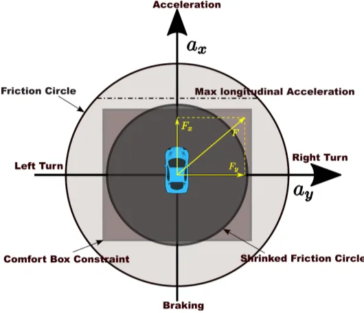
constraints are considered separately in the form ofcomfort box constraintsthat its upper boundaries need to be selected conservatively to prevent the total force from exceeding the friction force limits, the capacity of driving on the limits to deal with emergencies or pursue time efficiency is highly restricted. The difference of potential solution space of comfort box constraints and friction circle constraints is shown in Figure1. In addition, the reduction of friction coefficient in extreme weather conditions will shrink the friction circle and the original fixed comfort constraints may create one or several dangerous zones in solution space, as shown in Figure1, which will inevitably cause potential safety issues.

Figure 1.Friction Circles.

Dakibayet al. [4] exploited an aggressive speed planning method by numerically solving a nonlinear differential equation (NDE) about friction circle constraints and capping the speed profile with forward and reverse integration of accelerations results along the fixed path. Due to the approximation of solution of NDE, the full capacity of car is not explored. None of their results reaches exactly the friction circle. As the driving conditions are quite close to the limits, admissible room left for track errors is little. We argue that the smoothness of speed profiles still need to be considered to improve tracking performance of the controller for safety concerns (jerky speed profiles may result in overshooting and oscillation of controllers), even for aggressive driving scenarios, which did not appear in their solution.

Liuet al. [11] recently introduced a temporal optimization approach, optimizing time stamps for all waypoints along a fixed path with respect totime windowconstraints at each point, and then using a slack convex feasible set algorithm to solve it iteratively. Smoothness of the speed profile and time efficiency are taken into account in the problem formulation. However, thetime efficiencyis considered in an indirect way that optimizesIoDwith respect to a reference speed over the path. Their formulation leads to a highly nonlinear and non-convex problem and is solved by a local optimization method, thus only local optimality is guaranteed. They addressed some important constraints in Table1such assmoothness,time windowandcomfort boxconstraints in their formulation but left out the friction circle constraint, which does not fully exploit the acceleration capacity of the vehicle. In addition, since they optimized timestamps directly, we do not see a quick way to impose apath constraintor apoint constraintas a hard one to manipulate speed profiles.

3. Problem Formulation

Assuming a curvature continuous path has been generated by a hierarchical motion planning framework like [9,22], the speed planning is to find a time-efficient, safe, and smooth speed profile travelling along the fixed path with respect to both safety and performance constraints.

In order to solve the proposed problem, we optimize the performance criterions from three aspects, smoothnessJS, time efficiencyJT, and speed deviationJVfrom a desired speed, with others left as hard constraints or semi-hard constraints. We first introduce the path representation and explain the relationship of an arc-length parametrized path and a time parametrized path, then present mathematical expressions of all the constraints, and pose the optimization problem at the end.

3.1. Path Representation

The goal of speed planning is to find a speed profile along a fixed path. Since the path is known, we need to reconstruct the mapping between the known path and the speed profile, then represent the speed profile with parameters determined by the prescribed path. A rich set of parameterized path representations has been proposed in the literature, including B-spline [23,24], Bezier curve [25,26], clothoid [27,28], polynomial curve [29] and polynomial spiral [30,31]. It’s trivial to convert all the listed curve models to a simple waypoints representation, but not vice versa. In order to avoid the non-trivial converting between curve models, we use the general waypoints parametrization to represent a fixed path, with the orientation and curvature encoded implicitly by the path. Formally, we define a waypoints parametrized curve as a workspace path. A workspace path,r, of the body point, b, at the center of the rear axle with footprint,A, is defined asr:[0,sf]→R2. More specifically, we

consider the following arc-length parametric form in Cartesian coordinate system,

r(s) = (x(s),y(s)),s∈[0,sf], (1) wheresis the arc-length parameter along the path,x(s)andy(s)are the scalars along two orthogonal base axes respectively. The relationship between the arclengthsand the corresponding timetis formed as the functions= f(t), therefore the time parameterized workspace path ˜r(t) = (x˜(t), ˜y(t)),t∈[0,tf] can be easily acquired by substituting in fors.

Since the path,r(s), is known, the speed vector~vin Cartesian coordinates can be calculated as below1,

~v=r˙(s) =r0(s)f˙, (2)

1 _{The prime0and the dot·denote derivatives with respect to the arc-length,s, and the time,t, respectively for a curve}

wherer0(s)is the unit tangent vector of the pathr(s)atsthat represents the direction of the speed of a car by assuming no sliding, ˙f is the corresponding longitudinal speed of the car in ego frame. Letθ(s)

represent the heading of the car atsof the pathr, we get r0(s) =cos(θ(s)), sin(θ(s))

=x0(s),y0(s). (3) The acceleration vector~ain Cartesian coordinates system is

~a=r¨(s) =r00(s)f˙2+r0f¨, (4) where ¨f is the longitudinal acceleration andr00(s)is the principle normal vector of the path, which is also called the curvature vector. The 2-norm of ther00(s)is the scalar of the curvature

κ=kr

00

k. (5)

3.2. Vehicle Model and Vehicle Dynamics Constraints

path

R

x

0 y

y

x0

X Y

O

ego frame

global frame

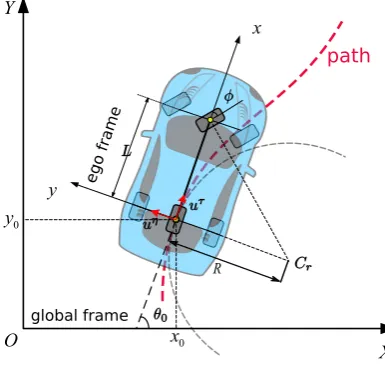
Figure 2.Single track car model.

Due to the non-holonomic dynamics of the vehicle system, the lateral motion and longitudinal motion are intrinsically coupled in a way that the car can not move laterally without longitudinal speeds. The lateral motion is explicitly expressed by the prescribed path. The longitudinal motion is the goal of this paper. In order to build the connection between them and describe the vehicle dynamics explicitly in the problem formulation, we employ the single track vehicle model [32] (see Figure2) to represent the actual vehicle kinematics and dynamics, which is widely used in motion planning research [9,19,22,30] and performs satisfactorily in practice [33]. The control force is defined asu= (uτ_,uη_{), whereu}η_{is the lateral force andu}τ_{is the longitudinal force in ego frame. The dynamics}

of the car are given by

Ru=m¨r, (6)

whereR=

"

cos(θ(s)) −sin(θ(s))

sin(θ(s)) cos(θ(s)) #

is the rotation matrix that maps forces from the ego frame to the

global Cartesian coordinate system,mis the mass of the car. We replace the ¨f with a functionα(s), ˙f2

with a functionβ(s)according to [2],

Then, ˙β(s) =2 ¨ff˙=2α(s)f˙=β0f˙. Thus,

β0(s) =2α(s),s∈[0,sf]. (8)

Therefore, equation (4), (6), and (8) form the dynamics constraints of cars.

3.3. Friction Circle Constraints

Given sufficient engine powers, it is well known that the traction power of the car produced by tires to drive the car is limited by frictions between tires and the road surface. The combination of lateral and longitudinal control forces that is able to be leveraged by cars should stay inside a friction circle to prevent slipping or car from running out of control, which is defined as below

kuk ≤µmg, (9)

whereµis the coefficient of friction between the tires and the road surface. The longitudinal force upper

boundary can be calculated according to the maximum longitudinal acceleration byuτ _≤m·aτ

max. This is only a necessary condition but not a sufficient condition to limit decision variables within the physical limits such as the nominal power. Take a driving case along a straight line for example, the speed will constantly increases to infinity if a fixed longitudinal force acts on the car and the path is long enough. But in reality, the max force that a plant system can provide is also limited by the nominal power of the engine. For most of the time, the actual power used by car systems is maintained below the nominal powerP, shown as below,

uτ_f˙_{≤P, (10)}

which also means, if the nominal power is reached, the driving force that a car is able to provide will decrease when the speed increases. This constraint is obviously nonlinear and non-convex. This issue ignored by [3] was first pointed out by Zhuet al. in [20], but they did not solve it and left it as future work. Here we provide our solution by adding an upper boundary constraint on speed profiles according to platform limits. It will prevent the speed from increasing without limits. Other constraints likepath constraints,boundary condition constraints, and thesmoothness objectivewill also restrict the upper boundary of speed profiles. By doing so, we partially address this issue without bringing in non-convexity to our problem formulation. Given these factors, the formal mathematical representation of friction circle constraints can be defined as below,

α(s),β(s),u(s)

∈

(

¨

r(s), ˙r2(s),u(s)

ku(s)k ≤µmg,

uτ_(s)≤m·aτ

max,

β(s)≤v2max

)

.

(11)

3.4. Time Efficiency Objective

Different from the approach used in [11] that optimizes deviation between the planned speed and desired speed to ensuring time efficiency implicitly, we optimize the total traveling time along the fixed path from 0 tosf directly like [2,3], which can be expressed asJT=T=R₀T1dt. Substitute the time variabletwith arclengthsand we get

JT =T=

Z f(t_f)

f(0)

1 ˙ fds=

Z s_f

0 β(s) −1

3.5. IoD Objective

In autonomous driving applications, users, a bahavior planning module or a task planning module may assign a reference speedvr for car to track. It is not a strict constraint like max speed thresholds or speed limits on the road that can’t be exceeded. Thus we introduce the integral of deviations between the planned speed and desired speed over the path as a soft constraint to measure this kind of performance, expressed as follows,

JV =

Z s_f

0 kβ(s)−v 2

rkds. (13)

Unlike Ref. [11] regarding it as the measurement of time efficiency, we call it the task soft constraint, which makes more sense according to the purpose it serves in the form of (13).

3.6. Smoothness Objective

Direct tracking of a minimum-time speed profile will lead to joint vibrations and overshoot of the nominal torque or force limits of actuators [34,35]. When this happens in autonomous driving cars, it most likely results in bad ride experience and unstable driving behaviors. In order to ensure a smooth speed profile for better tracking performance, reduced wear of power train systems and guarantee the ride comfort at the same time, the smoothness of the trajectory need to be considered. Since we assume a smooth and curvature-continuous path has been generated by a path planning module, we only consider the longitudinal jerk component of the trajectory. Formally speaking, jerk is the first derivative of acceleration in terms of timet, which also means the second derivative of velocity and the third derivative of position. According to (7) and (8), the jerkJ(s)of the speed profile can be calculated as follows,

J(s) =...f =α˙(s) =α0(s)f˙

=α0(s) q

β(s) = 1

2β

00_(s)q β(s),

(14)

which is nonlinear and non-convex. In fact, various smoothness metrics, including jerk, have been proposed to quantify the motion smoothness in literature [36,37]. However, the jerk objective brings in non-linearity and non-convexity, which makes our problem hard to solve, a better measurement which covers all the aspects we care about and also with good mathematical properties should be selected for the sake of fast convergence rate and optimality. Therefore we introduce apseudo jerk α0(s), which is the first derivative of acceleration with respect to the parameter arc-lengths, to the

problem to encourage smooth transitions between states. The smoothness objective is then defined as

JS =

Z s_f

0 kα

0_(s)k2_{ds, (15)}

which is convex. By minimizing the variation of acceleration in terms of parameter s, a smooth acceleration profile is preferred. By integrating the smooth acceleration alongs, the speed profile can be further smoothed.

3.7. Path Constraints

Path constraints can be defined as the following form,

ψ(s,x,u)≤0,∀s∈[0,sf], (16)

Rectangle Straight Line

Serrate

Figure 3.Different shapes of path constraints.

• Speed limits on certain segments of roads happen to be common driving scenarios in urban environments. The speed limits can not be exceeded by autonomous driving systems, or the driving system will violate the traffic regulations and be fined. The restrictions may happen along the whole path or just segments of the path, which is a little different from an overall speed threshold constraint and the IoD objective.

• A high-level planning system (i.e., behavior planning system, task planning system) may provide the upper boundary or lower boundary of the speed profile to a speed planner to make it behave well or satisfy certain task requirements. A speed planner has to plan a speed profile that stays in the prescribed region or below the envelope.

Both cases enforce hard constraints on speed profiles (state), which can not be ensured by using soft constraints of speed deviation presented in [11] or the IoD constraint described by us. The residues in soft constraint form can be minimized by optimization, but how the state (velocity) approaches the reference is not determined. Overshooting or oscillation may occur around the reference during the optimization. But a hard constraint like (16) is able to limit the “trace” of the system states strictly. More concisely, the specific constraints in our problem are expressed in the following form without involving control variables explicitly,

β(si)≤β¯(si),∀si∈[sm,sn], (17)

where ¯βis the upper boundary ofβats, 0≤sm≤sn≤sf andm<n. Three typical path constraints shapes of ¯β(si)are demonstrated in Figure3.

3.8. Boundary Condition Constraints

The boundary condition constraints specifically refer to the terminal constraints that can be generally represented by

g(sf,xf,uf)≤0, (18)

wherexf is terminal state variable anduf is the final control variable. More specifically, we impose the following constraint type,

α_sf ≤αsf ≤α¯sf β_s

f

≤βsf ≤β¯sf.

(19)

Withαs_f ≤α¯sf andβ_s f

≤_β¯_s

f, we can enforce either equality constraints (by “=”) or target set inequality

be guaranteed in this case. The other scenario occurs as a car tries to merge into an expressway from an entrance ramp, which needs to have the final speed fall in the speed limit range of the expressway. Other applications, such as keeping a fixed distance to the front car at the end of the path while matching the final speed with that of the front car can also be solved using this constraint in our framework. Such capacities are not present in [3,11]. If no strict boundary conditions on terminal states are required, the constraints can be deactivated by makingα_sf =−µg,β

sf

=0, ¯αsf =µg, ¯βsf =v2max.

3.9. Time Window Constraints

Time window constraints are represented as

ti=T(si)∈WT= (0,TU], (20) whereT(si) = R₀siβ(s)−12dsandT_U > 0. The constraint ensures that if the car passes the stations_i during the time windowWT, non-collision with other traffic participants is guaranteed. The time window,WT, can be acquired efficiently from a collision detection algorithm such as [39] with predicted trajectories of traffic participants in the workspace-time space. This type of constraint is very useful for handling time-critical tasks such as dynamic obstacle avoidance at certain points,si, along the path, and for arriving at the destination within the given max time duration. If no time window information about dynamic obstacles is available, this constraint can be relaxed by settingTU =∞.

3.10. Comfort Box Constraints

The comfort box constraint as another requirement of the ride comfort other than the smoothness, appears in a threshold form in the literature [7,9,11],

kaη_ik ≤aηc

kaτ

ik ≤aτc,

(21)

which is a hard constraint. Theaτ

c is the threshold for the longitudinal accelerations and decelerations. Theaηc is the threshold for lateral accelerations. This box form of constraints ensures comfort at the cost of mobility. The mobility may dramatically drop if the comfort acceleration thresholds are set too conservatively. The feasible region for optimization is limited within a rectangle inside the friction circle if (21) is present, as shown in Fig1. But when an emergency occurs, the planner may have to violate the comfort constraint to leverage more mobility of the car to generate a safe speed profile by ignoring the comfort constraint temporally instead of failing by satisfying it. With a hard constraint presented in the problem, there is no way to reach this goal. Thus we employ a penalty method with slack variables to soften the comfort box constraint [40,41], which makes it a “semi-hard” constraint. If the original optimization problem was

minimize

s J(s)

s.t. c(s)≤0,

(22)

an equivalent optimization problem using slack variables can be acquired as

minimize

s J(s) +λkσk

s.t. c(s)≤σ

0≤σ,

(23)

whereσis the slack variable that represent the constraint violations,λis the corresponding weight.

full mobility of cars and capacity of breaking the comfort box constraint to recover the feasibility when necessary. The exact expression of the semi-hard constraint is shown in (24).

3.11. Overall Convex Optimization Problem Formulation

Finally, the complete speed planning optimization problem over the fixed path is posed, which incorporates the full set of constraints presented above as,

minimize

α(s),β(s),u(s),

στ(s),ση(s)

J=ω1JT+ω2JS+ω3JV

+λ1kστ(s)k+λ2kση(s)k

s.t. (6), (8), (11), (17), (19), (20),

kα(s)k ≤aτ_c+στ(s),

kuη(s)

m k ≤a

η

c +ση(s),

0≤στ(s),

0≤ση(s),

(24)

where ˙r2(s) =r0(s)2β(s)and ¨r(s) =r0α(s) +r00β(s). Note thatα(s),β(s),u(s),στ(s),ση(s)are the

decision variables to optimize. The parametersω1,ω2,ω3,λ1,λ2∈R+are fixed in advance to suit the

particular application objectives. When parametersλ1,λ2are both set to zeros, theστ(s),ση(s)are

degenerated to constants zeros andaτ

c,aηc are set to infinity, which means the comfort box constraint is relaxed. The problem formulation we presented can be demonstrated to be convex as follows. For these readers who are not familiar with convex optimization, we refer them to [40,42] for details.

• For the objectives,JTis an integral of a negative power function and is therefore convex. JSis an integral of a squared power of absolute value and is therefore convex. JVis an integral of an identity power of absolute value and is therefore convex. So arekστkandkσηk. Asω1,ω2,ω3, λ1,λ2are all nonnegative,Jas a nonnegative weighted sum of convex functions, is convex.

• For (6), the dynamics equality constraint is affine inα,β,uand is therefore convex. For equality

constraints about decision variables (8), since the derivative is a linear operator, the relation betweenαandβis convex. For the inequality path constraint (17), β(si)is a sublevel set of convex set in the interval[sm,sn]and is thus convex. The equality and inequality constraints about boundary conditions (19) are linear constraints, thus convex. As theTiis an integral of a negative power function, therefore convex andTUis a fixed upper boundary, the time window inequality constraint (20) is a convex constraint.

• For the convex set constraint about the friction circle (11), the norm ofuis convex, upper bounds are fixed andv2

max is fixed, so the control set constraint is the intersection of three convex sets and is therefore convex.

• The comfort box constraints with slack variablesστandσηare second-order cone constraints

and convex.

Since the objectives are convex, equality contraints are affine and inequality constraints are convex, this optimization problem is convex [40]. The speed planning problem as stated is therefore an infinite-dimensional convex optimization problem.

4. Implementation

discretised points for all these numerical experiments in section5. For one segment of the path, we assume constant acceleration, which is also used in [2,3]. According to (8),β(s)can be expressed as,

β(s) =βi+ (s−si)(

βi+1−βi si+1−si

),s∈[si,si+1]. (25)

4.1. Discretization of JT, JS, and JV

Substitutingβ(s)−12 into (25) yields, JTi =

Z s_i+1

si

β(s)−

1 2ds

= Z s_i+1

si

βi+ (s−si)(

βi+1−βi si+1−si

) !−1

2 ds

= p 2·∆s

βi+

p βi+1

,

(26)

where∆s=si+1−siis a fixed arclength increment.

This integral can be approximated in the following form,

JT =2 N−1

∑

i=0

∆s

p

βi+

p βi+1

. (27)

For the smoothness term, we use finite differences to approximateα0(s), which yields

JS=

Z s_f

0 kα

0_(s)k2_ds

=

N−1

∑

i=0

kα(si+1)−α(si)

∆s k

2_∆s. (28)

TheJVcan be directly represented by

JV = N−1

∑

i=0

kβ(si)−v2rk∆s. (29)

4.2. Discretization of r0(s)and r00(s)

The discrete form representations of constraints are straight-forward to define, with the exception of the dynamics constraint (6), which involves first and second order derivatives ofr(s)with respect to the arclengths. We use finite differences to approximater0(s),

r0(s) = r(si+1)−r(si) si+1−si

, (30)

and a fourth-order Range-Kutta formula to approximater00(s),

r00(s) = r(si−2)−r(si−1)−r(si) +r(si+1)

2∆s2 . (31)

5. Numerical Results

In order to evaluate the performance and capabilities of the proposed speed planning model, we use a curvy example path from [3], as shown in Figure4, to conduct various challenging speed planning numerical experiments. To be fair, we implemented both our problem formulation and MTSOS in [3] in Julia [45] running on a PC with an Intel Xeon E3 processor at 2.8GHz and 8GB RAM in a Linux system and then compared our results with theirs to show the improvements and new capacities.

0.4

0.5

0.6

0.7

0.8

0.9

1.0

X/m

0.0

0.2

0.4

0.6

0.8

1.0

Y/

m

a smooth path

start

end

Figure 4.An example path from [3].

The used parameters are listed in the Table3. As it’s a proof of concept experiment, these parameters do not match those of the real platforms. But it does show the capacities of the speed planner from functional aspects. We will demonstrate the case studies using parameters from real platforms and dealing with real on-road driving scenarios in the next section.

Table 3.Parameter Values

Parameter Description Values Unit

m Mass of the car 0.1453 kg

µ Friction coefficient 0.70 1

g Acceleration of gravity 9.83 m/s2

aηc Longitudinal acceleration threshold for comfort 0.4·µg m/s2

aτ

c Lateral acceleration threshold for comfort 0.4·µg m/s2

aτ

max Max. longitudinal acceleration of the car. 0.5·µg m/s2

vmax Max. speed of the car. 1.8 m/s

As the friction circle constraint is the essence of the safety regarding vehicle dynamics, we enabled it for all the experiments below. We first run the MTSOS algorithm on the example path to generate the speed profile, accelerations and their distribution within the normalized friction circle as the baseline to compare with.

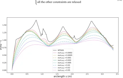
5.1. Smoothness

In this case, we show how the smoothness constraint of the our formulation affects the results and improve the performance. The initial speedpβ(0)of the car is a fixed point and assigned according to

enable onlyfriction circle constraint,time efficiency objective,smoothness objectiveby setting the parameters to

 



ω1=1,ω2(see Figure5), ω3=0

all the other constraints are relaxed (32)

0.0 0.5 1.0 1.5 2.0 2.5 3.0 3.5

arclength s (m)

0.25 0.50 0.75 1.00 1.25 1.50

V(

m

s

1

)

MTSOS ours, 2= 0.0002

ours, 2= 0.0005

ours, 2= 0.001

ours, 2= 0.002

ours, 2= 0.005

ours, 2= 0.01

ours, 2= 0.02

ours, 2= 0.05

Figure 5.Speed planning results with different coefficients of the smoothness objective.

The other constraints are all relaxed or ignored to remove side effects and highlight the effects of the smoothness objective term. The black curve presented in Figure5represents the speed profile generated by MTSOS[3] with only time efficiency objective and friction circles constraints. The colored curves depict our results using different coefficients for the smoothness objective. Multiple cusps are observed in the MTSOS’s result, which definitely increases the difficulty of tracking such a speed profile for controllers. Overshooting and oscillation may happen when tracking a non-smooth speed profile such as the black one. Instead, our method generates way more smooth speed profile without cusps while still keeping time efficiency in mind. With small coefficients for smoothness, the resulting speed profiles tend to stay close to the most time-efficient speed profile (the black one) while still maintaining high order continuity. As coefficients of smoothness increase, flatter slopes of speed profiles are encouraged, thus smoother speed profiles are generated. With this structure in hand, our method offers a way to balance the time efficiency performance and smoothness performance according to specific application requirements when necessary. We also demonstrated control efforts distribution of MTSOS, ours withω2=0.0002,ω2=0.002, andω2=0.02 using a normalized friction

1.00 0.75 0.50 0.25 0.00 0.25 0.50 0.75 1.00

a

a

Normalized acceleration Circle

Normalized Max Longitudinal Acceleration MTSOS

ours, 2= 0.0002 ours, 2= 0.002 ours, 2= 0.02

Figure 6.Friction circle for smoothness.

5.2. Boundary Condition Constraint

To demonstrate the capacity of boundary condition constraints, we carried out two set of experiments. In the first set of experiments, we compared the results with the following setting,

MTSOS         

time efficiency objective free final speed

friction circle constraint ours-A         

ω1=1,ω2=0,ω3=0

final speed constraintβ(sf) =0

all the other constraints are relaxed ours-B         

ω1=1,ω2=0.002,ω3=0

final speed constraintβ(sf) =0

all the other constraints are relaxed.

The caseA,Bin Figure7showed that our method is able to satisfy the final speed boundary condition while optimizing time efficiency (A) with a sharp slow-down slope or optimizing time efficiency and smoothness at the same time (B) with a flatter slow-down slope at the end. We conducted the second set of experiments with both time efficiency and smoothness objectives considered using same coefficients but with different type of boundary conditions,

ours-C               

ω1=1,ω2=0.05,ω3=0

inequality constraint:

0.22_≤

β(sf)≤0.32

all the other constraints are relaxed ours-D               

ω1=1,ω2=0.05,ω3=0

equality constraint:

β(sf) =0.52

all the other constraints are relaxed ours-E         

ω1=1,ω2=0.05,ω3=0

free final speed

all the other constraints are relaxed.

consistency of references and control stability. Since time efficiency is one of the objectives, it makes sense that the final speed of the caseCreached the upper boundary at the end when given a feasible range.

Neither MTSOS [3] nor [11] can deal with this case due to the lack of corresponding constraints. Adding a similar constraint to the MTSOS requires re-arrangement of the problem and non-trivial, error-prone changes to their customized solver. Regarding the final speed constraint as a soft one like [11] can not guarantee where and when the constraint is satisfied. Instead, our formulation and framework overcome above flaws.

0.0 0.5 1.0 1.5 2.0 2.5 3.0 3.5

arclength s (m)

0.0 0.2 0.4 0.6 0.8 1.0 1.2 1.4 1.6

V(

m

/s)

MTSOS, free end A- 2= 0, vf= 0

B- 2= 0.002, vf= 0

C- 2= 0.05, 0.2 vf 0.3

D- 2= 0.05, vf= 0.5

E- 2= 0.05, free end

0.2 0.3 0.4 0.5 0.6 0.7 0.8 0.9

Figure 7.Speed planning results with different end boundary conditions.

5.3. Path Constraint

0.0 0.5 1.0 1.5 2.0 2.5 3.0 3.5

arclength s (m)

0.0 0.2 0.4 0.6 0.8 1.0 1.2

V(

m

s

1

)

A-straight line path constraint B-rectangle path constraint C-serrate path constraint result without any path constraint result with A constraint result with B constraint result with C constraint

Figure 8.Speed planning results with different path constraints.

In this part, to show effects of path constraints, we conducted experiments with the friction circle constraint, time efficiency and smoothness objectives byω1=1,ω2=0.005,ω3=0. For the sake of

clarity, all the other hard constraints except path constraints are relaxed or ignored. For reference, a speed profile without any path constraint is generated using the given parameters (see the black curve in Figure8), which can be thought of as the original speed profile before imposing the path constraints. Then we enforced three types of path constraints to show the capacity of our method,

• rectangle shape (Bin fig.8) • serrated shape (Cin fig.8)

as seen in Figure8. The corresponding speed planning result is tagged using the same color with that of the path constraint. As shown in Figure8, the original speed profile was deformed by optimization according to path constraints and all the resulting speed profiles stayed below the corresponding path constraints strictly while still keeping smooth. This provides a powerful tool for users to customize the speed profiles according to their needs while guaranteeing high quality of solutions.

5.4. IoD task constraints

0.0 0.5 1.0 1.5 2.0 2.5 3.0 3.5

arclength s (m)

0.00 0.25 0.50 0.75 1.00 1.25 1.50 1.75

V(

m

s

1

)

MTSOS

A-desired speed profile B-desired speed profile result with A but no smoothness result with A and smoothness result with B but no smoothness result with B and smoothness

Figure 9.Speed planning results with desired speed in different shapes.

We evaluated effects of IoD task constraints using two different desired speed profiles (the dash-dot lineAand the dash-dash lineBin Figure9) to show the bahaviors of our planner. We first ran the MTSOS planner to generate the upper boundary of the speed profile for reference. For the desired speed profileAin Figure9, we consider the time efficiency objective and IoD objective only byω1=1, ω2=0,ω3=10 and relaxed all the other constraints to generate the speed profile, shown as the orange

curve in Figure9. The orange curve aligned well with the desired speed profile except for the part that the desired speed exceeds the limit of the friction circle. For the exceeding part, the orange curve stayed as close as possible to the desired speed but limited by the speed upper boundary constrained by the friction circle. This result uncovers the strong safety feature of our method. Moreover, taking the smoothness objective into consideration by makingω2=0.1, the quality of the speed profile is

further improved (see the green curve in Figure9). We also tested the IoD constraint against the totally feasible desired speed profile B using the same parameters setting with the previous experiment. The blue curve in Figure9depicted the planning result without considering smoothness. The resulting speed almost perfectly aligned with desired speed B. Similarly, the quality of the speed profile was significantly improved by add the smoothness objective (see light red curve in Figure9).

5.5. Time window Constraint

0.0 0.5 1.0 1.5 2.0 2.5 3.0 3.5

arclength s (m)

0.0 0.2 0.4 0.6 0.8 1.0 1.2

V(

m

s

)

1= 1, 2= 0.5, 3= 0, without time window constraint 1= 1, 2= 0.5, 3= 0, tsf 5s

1= 1, 2= 0.5, 3= 0, tsf 4s

Figure 10.Speed planning results with time window constraints.

a large coefficient for smoothness, the travel time at the end of the path reached 6.626 s. Note that the time window constraint in (20) can be enforced on any point along the path. For simplicity, we picked thesf point as the place where imposing the constraint. We added the time window constraint by limiting the arriving timeT(sf)at the end of the path to(0,TU], where theTU=5sfor case 1 and TU = 4sfor case 2 and solved them with respect to these constraints. The resulting speed profiles were shown as green and red curves for case 1 and case 2 in Figure10, respectively. The travel time at sf were listed in Table4and both time constraints were satisfied according to the data. The original speed profile (blue one) were regulated to meet the time window requirements. The resulting speed profile were clearly above the original speed profile. This is a powerful tool that makes us able to control the time arriving at a certain point of the path by using a large coefficient for smoothness then enforcing the time window constraint to compress the travel time below the upper boundary of the given time window. In this way, we can easily “stretch” or “compress” the travel time for a fixed path. An example of “stretching” the travel time can be found in section6.2case study.

Table 4.Time Window Constraints

Profile Coefficients Time Window Travel Time atsf

fig.10 (s) (s)

blue ω1=1,ω2=0.5 free 6.626

green ω1=1,ω2=0.5 tsf ∈(0, 5] 4.999 red ω1=1,ω2=0.5 tsf ∈(0, 4] 4.000

5.6. Semi-hard Comfort Box Constraint

To show the capacity of the semi-hard comfort box constraint, we conducted experiments with the following four different configurations,

case-A  



ω1=1,ω2=0,ω3=0

β(sf) =0,λ1=2,λ2=2

case-B  



ω1=1,ω2=0.05,ω3=0

β(sf) =0,λ1=2,λ2=2

case-C         

ω1=1,ω2=0,ω3=0

β(sf) =0,λ1=2,λ2=2

tsf ≤3.5s

case-D         

ω1=1,ω2=0.05,ω3=0

β(sf) =0,λ1=2,λ2=2

1.00 0.75 0.50 0.25 0.00 0.25 0.50 0.75 1.00

a

y

1.00

0.75

0.50

0.25

0.00

0.25

0.50

0.75

1.00

a

x

Normalized acceleration Circle

Normalized Max Longitudinal Acceleration

Comfort Box Constraint Bounds

1

= 1,

= 0,

= 0, t

free

= 1,

= 0.05,

= 0, t

free

= 1,

= 0,

= 0, t

3.5s

= 1,

= 0.05,

= 0, t

3.5s

Figure 11.The g-g diagram of semi-hard comfort box constraints.

0.0 0.5 1.0 1.5 2.0 2.5 3.0 3.5

arclength s (m)

0.2 0.4 0.6 0.8 1.0 1.2 1.4

V(

m

s

1

)

1= 1, 2= 0, 3= 0, tsf free

1= 1, 2= 0.05, 3= 0, tsf free

1= 1, 2= 0, 3= 0, tsf 3.5s

1= 1, 2= 0.05, 3= 0, tsf 3.5s

Figure 12.Speed profiles with semi-hard comfort box constraints.

The comfort acceleration thresholdsaτ _{and a}η _{are listed in Table3. For case A, we only took the}

in based on case A. The resulting speed profile is shown as the green curve in Figure12, which is smoother than previous one. The rationale behind this is that the smoothness term encourages gentle control efforts to keep smooth transitions between states. Thus the acceleration points of case B more focused around the center of the friction circle while still staying inside of the box, shown as green dots in Figure11. In order to demonstrate the “semi-hard” feature of our formulation, we imposes a time window constraint by making the final arriving timetsf ≤3.5s. With this constraint, the mobility

constrained by the box region is no longer enough to achieve the required time efficiency. In order to get a solution that satisfies the time window constraint, the optimization has to exploit the region that is within the friction circle but outside of the box. The results of the acceleration points distribution of case 3 (see cyan pentagons in Figure11) and case 4 (see pink pluses in11) proved our statements. The acceleration points were no longer limited within the box region. The corresponding speed curves were shown as the light red curve for case 3 and blue curve for case 4 in Figure12. This nice feature distinguishes our method from existing speed planning methods such as [7,9,11] that regard comfort box constraints as hard ones like (21). Their methods guaranteed the ride comfort at the expense of losing potential mobility. Limiting accelerations to the comfort box region dramatically reduces the solution space of the speed planning problem, which may lead to no solution when one does exist in certain situation. Our method, instead, turns the comfort constraint to a semi-hard constraint by leveraging penalty functions and slack variables. More precisely, when the region limited by the box constraint is able to provide the needed mobility to satisfy other hard constraints, the slack variables are reduced to zero and the penalty functions have no effects on the optimization. The comfort box constraint is equivalent to a hard constraint. But when the mobility provided by the box region is not enough to satisfy other hard constraints, slack variables increase and the penalty functions penalize the constraints violation. The comfort box constraint then is transferred to a soft constraint. By doing so, our method gives priority to the solution space in box region and leverages the outside region when necessary, which emphasizes comfort while keeping the solution space complete. To the best of our knowledge, none of the existing speed planning methods for autonomous driving has done this.

6. Case Study

In this section, we demonstrate three case studies to show how to combine constraints we present to solve distinct sets of speed planning problems raised in different real autonomous driving scenarios with parameters from the real platform like a Lincoln MKZ.

Table 5.Parameter Values

Parameter Description Values Unit

w Car width 2.45 m

l Car length 4.9 m

wb Car wheelbase 2.8448 m

tr Car track 1.5748 m

m Mass of the car. 1500.0 kg

µ Friction coefficient 0.7 1

g Acceleration of gravity 9.83 m/s2

aηc Longitudinal acceleration threshold for comfort 0.4·µg m/s2

aτ

c Lateral acceleration threshold for comfort 0.4·µg m/s2

aτ

max Max. longitudinal acceleration of the car 0.5·µg m/s2

vmax Max. speed of the car 30 m/s

6.1. Speed Planning for Safe Stop

fixed path road boundary obstacle

Figure 13.Safe stop scenario.

1.00 0.75 0.50 0.25 0.00 0.25 0.50 0.75 1.00

a

y

1.00 0.75 0.50 0.25 0.00 0.25 0.50 0.75 1.00

a

x

Normalized acceleration Circle

Normalized Max Longitudinal Acceleration Comfort Box Constraint Bounds

1= 1, 2= 0, 3= 0, 1= 0, 2= 0, vinit= 6m/s 1= 1, 2= 5, 3= 0, 1= 10, 2= 10, vinit= 6m/s 1= 1, 2= 5, 3= 0, 1= 10, 2= 10, vinit= 8m/s 1= 1, 2= 5, 3= 0, 1= 10, 2= 10, vinit= 12m/s

Figure 14.Friction circle for the safe stop scenario.

that considers the time efficiency, smoothness objectives, friction circle and final speed constraints by makingω1 = 1,ω2 = 5,β(sf) = 0. The initial speed of the car isvinit = 6m/s. The semi-hard comfort box constraints were not taken into consideration in this one. The corresponding results are shown in Figure14and Figure15in black color. The second experiment were carried out using the same parameters. In addition, the semi-hard comfort box constraints were added by settingλ1=10

0

5

10

15

20

25

30

arclength s (m)

0

2

4

6

8

10

12

V(

m

s

1

)

1

= 1,

= 0,

= 0,

= 0,

= 0, v

= 6m/s

1

= 1,

= 5,

= 0,

= 10,

= 10, v

= 6m/s

1

= 1,

= 5,

= 0,

= 10,

= 10, v

= 8m/s

1

= 1,

= 5,

= 0,

= 10,

= 10, v

= 12m/s

Figure 15.Speed profiles for the safe stop scenario.

comfort box constraints were not presented, the optimization uses more control efforts when cornering and stopping for the sake of time efficiency. Once comfort box constraints were added, the control efforts were limited into the box region when mobility is enough to use. Next, we conducted the next two experiments using the same setting with that of the green one except two different initial speed vinit=8m/s(cyan curves and dots) andvinit =12m/s(pink curve and dots). As shown in Figure14, when the initial speed increase to 8m/s, the region constrained by comfort box was still able to provide enough mobility to stop at the end. Thus all the acceleration points stayed inside the box region. But when the initial speed was increased dramatically to 12m/s, the optimization had to use more control efforts to stop in the end. In consequence, the box constraints are “softened” and acceleration points went beyond the box region to guarantee a safe stop. With the comfort box constraint as a hard one, the method can not get a solution in the last case.

6.2. Speed Planning Dealing with Jaywalking on a curvy road

fixed path road boundary

Figure 16.Jaywalking scenario.

Second, we considered a jaywalking scenario on a curvy road. The time window[t1=7s,t2=11s]

Pedestrian

Figure 17.S-T graph for the jaywalking scenario.

0

10

20

30

40

Arclength S (m)

0

5

10

V(

m

/s)

1

= 1,

= 5,

= 0,

= 10,

= 10, t

free

1

= 1,

= 15,

= 0,

= 10,

= 10, t

6.8s

1

= 1,

= 15,

= 0,

= 10,

= 10, t

11.2s

Figure 18.S-V graph for the jaywalking scenario.

the arrival time. Non-stop dynamic obstacle avoidance strategies may result in energy saving driving behavior or greatly reduced operation time in certain cases. As the pedestrian occupied the road between 7s and 11s ats=30malong the path, if our car reachess=30min the same time window, an accident may happen. Unfortunately, with the parameter settingω1=1,ω2=5,ω3=0,λ1=10,λ2=

10, our car will collide with the pedestrian, which is shown as the green curve in Figure17. Two strategies can be employed to avoid this failure. The first involves passing the potential collision point before the pedestrian arrives pointA, that is,ts=30m<=t1, which is shown as the blue car situation in

Figure16. The second involves passing the potential collision point just after the pedestrian passes pointB, that is,ts=30m >=t2, which is shown as a green car situation in Figure16. We solved this

problem using both strategies. By makingω1=1,ω2=15,ω3=0,λ1=10,λ2=10,ts=30m<=6.8s, we solved the former case and the corresponding results are demonstrated in color cyan in Figure17, Figure18, and Figure19. In practice, we may be not able to pass the barrier in time using the former strategy due to dynamics constraints of cars. The latter approach or a safe stop at a specified point along the path can be always employed to avoid collision. The latter approach is solved by setting

ω1=1,ω2=15,ω3=0,λ1=10,λ2=10,ts=30m<=11.2s. The results are presented in color pink in Figure17, Figure18, and Figure19. It should be noted that the second approach is an indirect method for avoiding collision in this scenario. We first stretch the time by increasing the coefficientω2from 5

1.00 0.75 0.50 0.25 0.00 0.25 0.50 0.75 1.00

a

y

1.00 0.75 0.50 0.25 0.00 0.25 0.50 0.75 1.00

a

x

Normalized acceleration Circle

Normalized Max Longitudinal Acceleration Comfort Box Constraint Bounds

1= 1, 2= 5, 3= 0, 1= 10, 2= 10, ts = 30m free 1= 1, 2= 15, 3= 0, 1= 10, 2= 10, ts = 30m 6.8s 1= 1, 2= 15, 3= 0, 1= 10, 2= 10, ts = 30m 11.2s

Figure 19.Friction circle for the jaywalking scenario.

Potential Collision Point

Figure 20.Freeway entrance ramp merging scenario.

0 20 40 60 80 100 120

Arclength S (m)

5 10 15 20

V

(m

s

1

)

1= 1, 2= 5, 3= 0, 1= 10, 2= 10, tsf free

1= 1, 2= 5, 3= 0, 1= 10, 2= 10, tsf 8.5s

Figure 21.S-V graph for freeway entrance ramp merging.

6.3. Speed planning for Freeway Entrance Ramp Merging

Finally, we demonstrate a freeway entrance ramp merging scenario. The oncoming yellow car is driving in around 20m/s. The arrival timetA=8.5sat merging pointAin Figure20is given by the dynamic obstacle prediction or V2V communication module. The initial speed of the autonomous driving car is 4m/s. With the parameter setting ω1 = 1, ω2 = 5, ω3 = 0, λ1 = 10, λ2 = 10,

20m/s ≤ vf ≤ 22m/s, the arrival time tsf at positionB of the autonomous car provided by the

merging point

Figure 22.S-T graph for the freeway entrance ramp merging scenario.

corresponding S-T graph is depicted in Figure22in green. The trajectory of the on-coming car is shown as the black curve in Figure22. The scenario is designed such that the autonomous car would collide with the oncoming vehicle in the conflict zone if the oncoming car does not yield. To avoid the risk, we enforce a time window constraint at the end of the path, based on the previous parameter setting by makingtf ≤8.5s. In this way, the autonomous vehicle has already reached positionBby the time the oncoming vehicle arrives positionA, which also keeps a safe distance between the two vehicles. Further, the final speed of the autonomous car is constrained to be no less than that of the oncoming vehicle, which ensures that the safety is guaranteed. The corresponding solution is depicted by the cyan curve in Figure21and Figure22. The exact arrival time at the end is 8.5s.

7. Conclusions

In this paper, we summarize and categorize the constraints needed to solve various speed planning problems in different scenarios as therequirementsfor speed planners design andmetricsto measure the capacity of the existing speed planners for autonomous driving. Keeping these requirements and metrics in mind, we present a more general, complete, flexible speed planning mathematical model including time efficiency, friction circle, vehicle dynamics, smoothness, comfort, time window, boundary condition, speed deviations from desired speeds and path constraints for speed planning along a fixed path. The proposed formulation is able to deal with many more speed planning problems raised in different scenarios in both static and dynamic environments while providing high-quality, time-efficient, safety-guaranteed, dynamic-feasible solutions in one framework compared to existing methods. By considering the comfort box constraints as a semi-hard constraint and implementing it with slack variables and penalty functions in optimization, we emphasize comfort performance while guaranteeing fundamental motion safety without sacrificing the mobility of cars. We demonstrate that our problem preserves convexity with all these constraints added, therefore the global optimality is guaranteed. We conduct a range of numerical experiments to show how every constraint affects the speed planning results and showcase how our method can be used to solve speed planning problems by providing several challenging case studies in both static and dynamic environments. These results have depicted that the proposed method outperforms existing speed planners for autonomous driving in terms of constraint type covered, optimality, safety, mobility and flexibility.

Acknowledgments:We would like to thank Mr Assylbek Dakibay for proof reading the manuscript.

Author Contributions:The work presented here was carried out in collaboration among all authors. All authors have contributed to, seen and approved the manuscript. Yu Zhang conceived of the work, realized the algorithms, performed the experiments, analyzed the data and wrote the manuscript. Steven L. Waslander reviewed and revised the manuscript and give some important advice. Huiyan Chen, Steven L. Waslander, Guangming Xiong, Tian Yang, Sheng Zhang and Kai Liu provided many useful suggestions for the work and made great efforts with respect to the paper revision. Tian Yang and Sheng Zhang designed the scenarios for case studies and provided corresponding figures.

References

1. Kritayakirana, K.; Gerdes, J.C. Autonomous vehicle control at the limits of handling. International Journal of Vehicle Autonomous Systems2012,10, 271–296.

2. Verscheure, D.; Demeulenaere, B.; Swevers, J.; De Schutter, J.; Diehl, M. Time-optimal path tracking for robots: A convex optimization approach. IEEE Transactions on Automatic Control2009,54, 2318–2327. 3. Lipp, T.; Boyd, S. Minimum-time speed optimisation over a fixed path. International Journal of Control2014,

87, 1297–1311.

4. Dakibay, A.; Waslander, S.L. Aggressive Vehicle Control Using Polynomial Spiral Curves. IEEE International Conference on Intelligent Transportation Systems (ITSC); , 2017.

5. Cabrera, J.A.; Castillo, J.J.; Pérez, J.; Velasco, J.M.; Guerra, A.J.; Hernández, P. A procedure for determining tire-road friction characteristics using a modification of the magic formula based on experimental results.

Sensors (Switzerland)2018,18.

6. Yunta, J.; Garcia-Pozuelo, D.; Diaz, V.; Olatunbosun, O. A Strain-Based Method to Detect Tires´Loss of Grip and Estimate Lateral Friction Coefficient from Experimental Data by Fuzzy Logic for Intelligent Tire Development. Sensors (Switzerland)2018,18.

7. Li, X.; Sun, Z.; Cao, D.; He, Z.; Zhu, Q. Real-time trajectory planning for autonomous urban driving: Framework, Algorithms, and Verifications. IEEE/ASME Transactions on Mechatronics2016,21, 740–753. 8. Gu, T.; Snider, J.; Dolan, J.M.; Lee, J.w. Focused trajectory planning for autonomous on-road driving. IEEE

Intelligent Vehicles Symposium (IV), 2013, pp. 547–552.

9. Gu, T. Improved Trajectory Planning for On-Road Self-Driving Vehicles Via Combined Graph Search, Optimization & Topology Analysis. PhD thesis, Carnegie Mellon University, 2017.

10. Gu, T.; Atwood, J.; Dong, C.; Dolan, J.M.; Lee, J.W. Tunable and stable real-time trajectory planning for urban autonomous driving. IEEE/RSJ International Conference on Intelligent Robots and Systems (IROS), 2015, pp. 250–256.

11. Liu, C.; Zhan, W.; Tomizuka, M. Speed profile planning in dynamic environments via temporal optimization. IEEE Intelligent Vehicles Symposium (IV), 2017, pp. 154–159. doi:10.1109/IVS.2017.7995713. 12. Wei, J.; Dolan, J.M.; Litkouhi, B. Autonomous vehicle social behavior for highway entrance ramp

management. IEEE Intelligent Vehicles Symposium (IV), 2013, pp. 201–207.

13. Xie, Y.; Zhang, H.; Gartner, N.H.; Arsava, T. Collaborative merging strategy for freeway ramp operations in a connected and autonomous vehicles environment. Journal of Intelligent Transportation Systems2017,

21, 136–147.

14. Serna, C.G.; Ruichek, Y. Dynamic speed adaptation for path tracking based on curvature information and speed limits. Sensors (Switzerland)2017,17.

15. Li, B.; Shao, Z. Simultaneous dynamic optimization: A trajectory planning method for nonholonomic car-like robots. Advances in Engineering Software2015,87, 30–42.

16. Ziegler, J.; Bender, P.; Dang, T.; Stiller, C. Trajectory planning for Bertha – A local, continuous method. IEEE Intelligent Vehicles Symposium (IV), 2014, pp. 450–457.

17. Schwarting, W.; Alonso-Mora, J.; Pauli, L.; Karaman, S.; Rus, D. Parallel autonomy in automated vehicles: Safe motion generation with minimal intervention. IEEE International Conference on Robotics and Automation (ICRA), 2017, pp. 1928–1935.

18. Ziegler, J.; Stiller, C. Spatiotemporal state lattices for fast trajectory planning in dynamic on-road driving scenarios. IEEE/RSJ International Conference on Intelligent Robots and Systems (IROS), 2009, pp. 1879–1884.

19. McNaughton, M.; Urmson, C.; Dolan, J.M.; Lee, J.W. Motion planning for autonomous driving with a conformal spatiotemporal lattice. IEEE International Conference on Robotics and Automation (ICRA), 2011, pp. 4889–4895.

20. Zhu, Z.; Schmerling, E.; Pavone, M. A convex optimization approach to smooth trajectories for motion planning with car-like robots. IEEE 54th Annual Conference on Decision and Control (CDC), 2015, pp. 835–842.

21. Kuwata, Y.; Karaman, S.; Teo, J.; Frazzoli, E.; How, J.; Fiore, G. Real-Time Motion Planning With Applications to Autonomous Urban Driving. IEEE Transactions on Control Systems Technology2009,