FastPRP: Fast Pseudo-Random Permutations for Small Domains

FastPRP: Fast Pseudo-Random Permutations

for Small Domains

Emil Stefanov

[email protected]

Elaine Shi

[email protected]

ABSTRACT

We propose a novelsmall-domain pseudo-random permuta-tion, also referred to as a small-domain cipher or small-domain (deterministic) encryption. We prove that our con-struction achieves “strong security”, i.e., is indistinguishable from a random permutation even when an adversary has observed all possible input-output pairs. More importantly, our construction is 1,000 to 8,000 times faster in most realistic scenarios, in comparison with the best known con-struction (also achieving strong security). Our implementa-tion leverages the extended instrucimplementa-tion sets of modern pro-cessors; and we also introduce a smart caching strategy to freely tune the tradeoff between time and space.

1.

INTRODUCTION

Pseudo-random permutations (PRPs), also referred to as block ciphers, are at the foundation of modern cryptography. This paper investigates the problem of constructing pseudo-random permutations over asmall domain.

Applications of small-domain PRPs. First proposed and studied by Black and Rogaway [7], small-domain PRPs are useful in a variety of application scenarios. For example, they are used in cryptographic constructions (e.g., Oblivious RAMs [9, 18]) for randomly reordering (permuting) a list of items. They can be used to generate pseudo-random unique tokens (e.g., product serial numbers) in a specific format. They can also be used to encrypt data in a small domain, such as encrypting a 9-digit social security number into an-other 9-digit number. Because of this, a small-domain PRP is also commonly referred to as asmall-domain cipher or format-preserving encryption(FPE). FPE has been a useful tool in encrypting financial and personal identification infor-mation, and transparently encrypting information in legacy databases.

Challenges and requirements.The construction of small-domain PRPs presents unique technical challenges. First, note that applying a large-domain PRP such as a 128-bit

Permission to make digital or hard copies of all or part of this work for personal or classroom use is granted without fee provided that copies are not made or distributed for profit or commercial advantage and that copies bear this notice and the full citation on the first page. To copy otherwise, to republish, to post on servers or to redistribute to lists, requires prior specific permission and/or a fee.

Copyright 20XX ACM X-XXXXX-XX-X/XX/XX ...$10.00.

AES and then projecting back into the domain D would destroy permutivity. In addition, there are several other challenges as suggested below.

• Arbitrary domain size. In this paper, we wish to con-struct small-domain PRPs that support arbitrary do-main sizes, as opposed to fixed dodo-main size, such as 16-bit or 32-bit.

• Non-standard security requirement. Standard large-domain PRPs over {0,1}`

typically achieve security against an adversary who can issue up to q 2` queries. With small-domain PRPs, the adversary might be able to exhaust all possible plaintext-ciphertext pairs. Our goal is to design a small-domain PRP that can withstand up to N queries from the adversary1_{. In} other words, we require the small-domain PRP to be indisitinguishable from a random permutation, even to an adversary who has observed allNpossible plaintext-ciphertext pairs.

• Efficient point-wise evaluation with small time and space. Another requirement is that the small-domain PRP should allow efficient point-wise evaluation. For ex-ample, one should be able to evaluate the outcome of the PRP over any inputxin time and spacesublinear inN.

1.1

Our Results and Contributions

As shown in Table 1, existing small-domain PRP schemes are either entirely based on empirical (but not provable) security [3, 4, 16] or fall short of security and only have prov-able security for a small number of adversary queries [7, 13] (q N). Recently, Granboulan and Pornin [10] propose a novel small-domain PRP construction that can withstand

N queries, and has provable security. While their scheme achieves non-trivial asymptotics, namely O((logN)3) time and O(logN) space per invocation, it is generally consid-ered to be impractical [6] due to the need to sample from the hypergeometric distribution, which is a heavy-weight op-eration.

We take an unconventional approach to solve this prob-lem. We observe that asymptotic performance is not the best metric to optimize for these small domain problems – 1

Note that in some earlier works, this same notion of security was also referred to as “withstandingN−2 queries”, in the sense that the adversary cannot predict the remaining two outputs with probability more than 1

2, even after observing

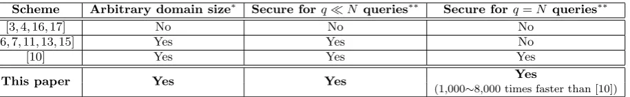
Scheme Arbitrary domain size∗ Secure forqN queries∗∗ Secure forq=N queries∗∗

[3, 4, 16, 17] No No No

[6, 7, 11, 13, 15] Yes Yes No

[10] Yes Yes Yes

This paper Yes Yes Yes

(1,000∼8,000 times faster than [10])

*: Note that cycle-walking can be used in general to achieve arbitrary domain size, but is usually quite costly.

**: By “secure”, we mean provably (rather than empirically) indistinguishable from a random permutation even when the adversary has seen anyqpossible input-output pairs.

Table 1: Comparison with related work

since asymptotic analysis by nature characterizes the per-formance of algorithms under very large inputs. There-fore, instead of proposing a construction that is asymptot-ically better, we propose one that is asymptotasymptot-ically worse –O(√NlogN) in both time and space – but is 1,000 to

8,000times faster than the best existing scheme [10] for the most common use cases (domains of sizes up to N = 232 items). Our construction is currently by far the most prac-tical construction for most realistic scenarios. In addition, our construction can withstand up toN queries by the ad-versary, and its security formally reduces to the security of the underlying AES function, which is used to generate the pseudo-random source needed by our construction.

1.2

Technical Highlights

No costly sampling from hypergeometric distribu-tions. One approach taken by Granboulan and Pornin [10] to construct a random permutation is to recursively parti-tion (at random) a set of N items into two equally sized sets, until each set has size 1. The task of partitioning a set ofN items into two equally sized sets can essentially be transformed into the task of generating N random bits of which exactly N₂ are 0 and N₂ are 1. Generating this bit-string turns out to be a difficult problem because it seems to require sampling from the hypergeometric distribution with very high accuracy in order to preserve security.

We observe that it is possible to avoid the costly sam-pling by relaxing the requirements and allowing there to be slightly more ones or zeros in the bitstring. In our construc-tion, each bit is randomly and independently generated and so the total number of ones or zeros is a distribution centered on N

2.

Leveraging modern processor features. Our imple-mentation is highly optimized and takes advantage of mod-ern processors’ extended instructions, includingAES instruc-tions and thePOPCNTinstruction. These advanced x86-64 in-structions are widely available on most modern server, desk-top, and laptop processors.

Even though existing algorithms can also be modified to use those instructions, they do not benefit nearly as much. In fact, we modified the code of [10] to use those hardware instructions and our algorithm is still thousands of times faster.

Tunable time-space tradeoff.We propose a smart caching strategy (Section 4) to cache and reuse intermediate com-putation results – specifically, counters, as described in Sec-tion 4 – allowing us to evaluate the permutaSec-tion inO(√NlogN) time and space.

Our scheme is dynamically adjustable to the amount of

cache available. Specifically, at run-time, if the amount of available memory changes, our scheme can dynamically ad-just and maximally leverage the available memory to mini-mize the computation time.

Finally, note that although our construction requiresO(NlogN) initial setup cost, in reality, since N is small (e.g., N = 232_{), the actual setup time of our algorithm is comparable} to cost of RSA key generation. This again demonstrates that asymptotics is the wrong metric to optimize for small domain problems.

1.3

Related Work

The problem of construct a domain PRP or small-domain cipher was initially studied by Black and Rogaway [7].

One class of approaches is balanced or unbalanced Feistel-based constructions [6,11,13,15]. However, these approaches do not have proven security against up toN queries when applied to small domains. Let N = 2n denote the size of the domain. For balanced cipher, Luby and Racoff [11] showed that 4 rounds can provide security to nearly 2n/4 queries. Maurer and Pietrzak [12] show that r rounds of balanced Feistel could withstand about 2n/2−1/r queries. Patarin [14, 15] shows that 6 rounds is enough to withstand about 2n/2queries. Morriset al. analyze the security of the Thorp shuffle [13], which is a maximally unbalanced Feis-tel network. They show that the Thorp shuffle with O(r) rounds is resilient up to 2n(1−1/r) queries.

Another class of approaches isde novo constructions [3, 4, 16, 17]. These constructions have empirical, but not prov-able security. Some of them only work for fixed length block ciphers. Moreover, due to lack of provable security, signifi-cant attacks were found with the TEA construction, leading to the hacking of Microsoft XBox console.

Small-domain ciphers are a special case of format-preserving encryption, which was informally described by Brightwell and Smith [8], named by Spies, and recently received a more systematic treatment by Bellare and Ristenpart [5].

Table 1 compares our work against related work in this space.

2.

PROBLEM DEFINITION

We first formally define pseudo-random permutations and their security requirement.

Definition 1 (CCA-secure PRP). LetD:={0,1, . . . , N− 1}denote a finite domain of elements. LetK:={0,1}k

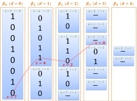
Figure 1: Example of the permutation algorithm.

• For any K ∈ K, PRP(K,·) is a one-to-one function fromDtoD, and can be evaluated in polynomial time.

• For any t-time algorithm A making at least q oracle queries,

Pr

k←K$

[APRP(K,·),PRP−1(K,·)= 1]− Pr

p←P$

[Ap,p−1= 1]≤

whereP denotes the family of all permutations forD.

In particular, in this paper, we would like to construct pseudo-random functions a small domainD:={0,1, . . . , N− 1}that aresecure against up toq=N queries.

Our construction leverages a Pseudo-Random Function (PRF) for large domains, such as AES. We formally define PRF as below.

Definition 2 (Secure PRF). LetPRF:{0,1}k_×{0 ,1}m

→ {0,1}n_{denote a function that takes in a key from{0,1}}k_,

and a string from{0,1}m

, and outputs a string in{0,1}n

. We say thatPRFis a(t, q, )-pseudo-random function, if

• For anyK∈ K,PRF(K,·)can be evaluated in polyno-mial time.

• For any t-time algorithm A making at least q oracle queries,

Pr

k←K$

[APRF(K,·)= 1]− Pr

f←F$

[Af = 1]≤

whereFdenotes the family of all functions from{0,1}m

to{0,1}n

.

3.

ALGORITHM

3.1

Intuition

Suppose that we would like to randomly permuteN ele-ments from a domainD:={0,1, . . . , N−1}. The permuta-tion can be done in the following manner:

• Choose a random bitβ[i]∈R{0,1}for everyi∈ D.

• LetS0 :={i

i∈ Dandβ[i] = 0}denote the set of

elements whose β[i] values are 0, let S1 := {i

i ∈

Dandβ[i] = 1}denote the set of elements whoseβ[i] values are 1.

Place the setS0ahead ofS1 in the final permutation. • Recurse and permute both setsS0 andS1.

The above randomized algorithm generates a random per-mutation over the domain D:={0,1, . . . , N−1}. For the formal proof of this, please refer to Section 3.5. To con-struct a pseudo-random permutation, one can simply use a pseudo-random source in place of the random bits fed to the algorithm. For instance, we can useAESK(·) to generate the

pseudo-random bits ofβ to obtain a keyed pseudo-random permutation where the secret key isK.

Example. Figure 1 illustrates the informal algorithm de-scribed above, using a small domain example, where D:= {0,1, . . . ,7}. To find the outcome of the pseudo-random permutation on the inputx= 7, one first assigns a random bit to each of the elements inD:={0,1, . . .7}. The vector of these random bits form the bitstring β0. Since x = 7 gets assigned the random bit 0, it will be placed in the top partition. Now this process is recursively applied to the top partition, where the element was mapped to, until a parti-tion of size 1 is reached. At that point, this pseudo-random permutation algorithm determines that the final location of input 7 is 2.

3.2

An Alternative View of the Algorithm

• First, for each input i ∈ {0,1, . . . , N −1}, assign a randomO(logN)-bit numberρito elementi. (For ex-ample, in Figure 1, the random number assigned to the element 7 is represented by the bits on the highlighted red path.)

• Next, sort alli’s based on theirρivalues. With high probability, allNelements will be assigned a uniqueρi, which determines a unique ordering of allN elements. It is not hard to see that the above-mentioned procedure outputs a random permutation of all elementsi∈ {0,1, . . . , N− 1}.

Moreover, it is not hard to see that Figure 1 effectively implements this above procedure, where the sorting is ac-complished through a radix-sort process. In particular, in the first step of the recursion, the inputs are sorted based on the first bit of each ρi. We then recurse on this, and in depthdof the recursion, thed-th bit is being sorted.

Based on this alternative view of the algorithm, it is not hard to see that if the bit-strings β0, β1, . . . are generated at random, then the above process yields a random permu-tation. Similarly, if the bit-stringsβ0, β1, . . . are generated from a pseudo-random sequence, the above process yields a pseudo-random permutation. The formal security state-ments and proofs are presented in Section 3.5.

3.3

Notations

Pseudo-random bitstringsβd. The bitstringsβdare in-dexable arrays of pseudo-random independent bits. Each bitstring isN bits long. The value of bitiof bitstringβdis denoted asβd[i].

Bit counters C0 and C1. The number of zeros in R = {βd[α],βd[α+ 1],. . .,βd[α+x]}is denoted asC0(βd, α, x). Similarly, the number of ones is denoted asC1(βd, α, x). The setRis called the input range ofC0andC1.

Bit locatorsC−01andC

−1

1 . The index of thek’th zero bit in

R={βd[α], βd[α+ 1], . . .}is denoted asC−1

0 (βd, α, k). Simi-larly, the index of thek-th one bit is denoted asC−₁1(βd, α, k). The setRis called the input range ofC−01andC

−1 1 .

3.4

Detailed Construction

Recall that we wish to construct a small-domain pseudo-random permutation, PRP : K × D → D, where D := {0,1, . . . , N−1} represents the domain, andK:= {0,1}k

represents the key space.

Generation of pseudo-random source. The Permute andUnpermutealgorithms below require pseudo-random bits as inputs. For notational convenience, we will divide these pseudo-random bits into bitstrings, denoted as{β0, β1, . . . ,}, where eachβi∈ {0,1}N

is a bitstring of lengthN.

These pseudo-random bits are generated with the keyK∈ Kto the small-domain PRP, by applying theAESfunction:

S=AESK(0)||AESK(1)||AESK(2)||. . . , (1)

In particular,β0 will be the firstN bits ofS,β1 will be the nextN bits ofS, and so on.

Permute. To compute PRP(K, x), where K ∈ K, x ∈ M, simply call the recursive function shown in Figure 2 with Permute(x,0, N,0). Specifically, the pseudo-random bits β0, β1, . . . required in this algorithm are generated as in Equation 1 above.

Figure 1 is an example walk-through of this algorithm for a small domainD:={0,1, . . . ,7}. In Section 7, we show that the algorithm will terminate within depthdofO(logN) with high probability.

Unpermute. To compute PRP−1(K, y), where K ∈ K,

y∈ M, simply call the recursive function shown in Figure 3 withUnpermute(y,0, N,0). Specifically, the pseudo-random bitsβ0, β1, . . .required in this algorithm are generated as in Equation 1 above.

Since Unpermute is the inverse function of Permute, and shares the same recursion tree asPermute, its depth is also bounded byO(logN) with high probability (Section 7).

3.5

Security Analysis

The alternative view on the algorithm described in Sec-tion 3.2 immediately gives us the following theorem:

Theorem 1 (Random permutation). Assuming the bit vectorsβ0, β1, . . . ,are chosen at random, where each bit rep-resents the outcome of an indenpendent random coin flip. The algorithm described in Figure 2 yields a perfectly ran-dom permutation over elements inD={0,1, . . . , N−1}.

Proof. As mentioned in Section 3.2, an alternative view of the algorithm is to assign a randomk-bit numberρi to each elementi∈ D, wherek =O(logN) with overwhelm-ing probability (see Theorem??). Then, it is not hard to see that the permutation algorithm described in Figure 2 is

essentially performing a radix sort on these elements based the binary representation of theirρinumbers.

Clearly, the process of assigning sufficiently large (k =

O(logN) with high probability) random numbers to each element and sorting these elements based on these random numbers would give us a random permutation. And since our algorithm is equivalent to this process, where the sorting part is achieved through a radix sort, the algorithm in Fig-ure 2 results in a random permutation, assuming the bits

β0, β1, . . . are chosen independently and uniformly at ran-dom.

Theorem 1 assumes that the bit-strings β0, β1, . . . , are chosen at random. Instead, if these bit-strings are generated pseudo-randomly fromAES, one can show that the resulting small-domainPRPis “at least as secure as”AES. To prove this, one has to ensure that the permutation algorithm has bounded depth, such that the bit-stringsβ0, β1, . . . ,can be obtained from a bounded number of AES invocations. In particular,kinvocations ofAESwould lead to a multiplica-tive factor ofk in the advantage of the adversary.

Corollary 1. Assume the bit vectorsβ0, β1, . . . are ob-tained from a pseudo-random sequence, generated by apply-ing an`-bitAESas in Equation 1. Typically,`= 128or256 bits.

Suppose the underlying AES is a (t, q, )-pseudo-random permutation, where q ≥4Nlog4

3N/`. Then, the algorithm described in Figure 2 yields a(t, N, +exp(−q`

8N)·N

)-pseudo-random permutation.

In particular, the security loss term exp(−₈q`<sub>N</sub>)·N is due to the failure probability that the algorithm needs to make more thanqqueries to the AES oracle. This happens when the algorithm completes in more than q`_N rounds.

To interpret the above corollary under realistic parametriza-tions, we give the following back-of-the-envelope calcula-tion. For example, imagine we use 256-bit AES, and suppose

N = 231 or smaller. Due to the birthday paradox, assume that the security of AES as a PRF is roughly defined by the relation ' q2

2256. When q = 2

34 _{≥ 4Nlog}

4

3N/`, the security loss of AES as a PRF under q queries is roughly

' 1

2188, the additional security loss of the resulting small-domain PRP is exp(−q`_8N)·N < 1

2338.

Proof. (of Corollary 1.) Suppose that there exists an adversary Awho can break the small-domain permutation PRP. We now leverage this adversaryAto construct a sim-ulator B which can distinguish AES from a truly random function.

Basically,Asubmits a sequence ofPRPorPRP−1_queries to B, and B will simulate the small-domainPRP function, and evaluate the outcomes of the PRPfunction, and its in-verse PRP−1 _{for A. To do this, B obtains its bit-strings}

β0, β1, . . .from an oracle, which either is generated from the AESfunction or a pure random function.

Due to Theorem 2, the probability that the process com-pletes in more thanc=q`_N ≥4 log4

3Nrounds is bounded by

N·exp(−c/8) =N·exp(−₈q`<sub>N</sub>). Therefore, with probability 1−exp(−q`

8N)·N,Bonly has to makeqor fewer queries to

the oracle. If, however, this fails,Bsimply aborts.

Permute(x, α, `, d): 1: if `= 1then

2: returnα

3: end if

4: if βd[α+x] = 0then

5: x0←C0(βd, α, x)

6: returnPermute(x0, α,C0(βd, α, `), d+ 1) 7: else

8: x0←C1(βd, α, x)

9: returnPermute(x0, α+C0(βd, α, `),C1(βd, α, `), d+ 1) 10: end if

Figure 2: Permutation algorithm (encryption).

Unpermute(y, α, `, d): 1: if `= 1then

2: return0 3: end if

4: if y <C0(α, `, d)then 5: y0←y

6: x0←Unpermute(y0, α,C0(βd, α, `), d+ 1) 7: returnC−1

0 (βd, α, x

0

+ 1) 8: else

9: y0←y−C0(βd, α, `)

10: x0←Unpermute(y0, α+C0(βd, α, `),C1(βd, α, `), d+ 1) 11: returnC−₁1(βd, α, x0+ 1)

12: end if

Figure 3: Inverse permutation algorithm (decryption).

a random permutation, thenBwould be able to distinguish whether the oracle is a pseudo-random source generated from AES or a pure random source, thereby breaking the security ofAES.

4.

CACHING COUNTERS

The scheme will be very slow if we implement thePermute andUnpermutealgorithms exactly as shown in Figures 2 and 3. The reason is that a naive implementation of theC0,C1, C−1

0 , andC

−1

1 functions cause a linear scan of large ranges ofβd. The total length of the scanned regions is O(N), so a naive implementation of Permuteand Unpermute would result inO(N) running time, which is too slow in practice.

We reduce the time complexity ofPermuteandUnpermute to O(√NlogN) with O(√NlogN) amount of space, by caching a small number of intermediate counters ofβ with a granularitys(called the cache stride).

Definition 3 (Cache Strides). The cache stride

de-termines the interval at which the values ofC1(·)are cached. With a cache strides, the values ofC1(βd,0, s·i)are cached ford= 0,1, . . . , O(logN)andi= 1,2, . . . , N/s.

Generating the cache takesO(NlogN) time, but is per-formed only once at initialization. In our experiments in Section 6.1, we show that it can be done reasonably fast (less than 10−6 _{seconds forN <2}15_{to 2.3 seconds forN= 2}31_). After this one-time initialization, we can reuse the cache to evaluate multiple “ciphertexts” with the same key.

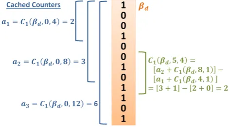
Figure 4: Using cached values of C1(·) to efficiently

compute arbitrary values of C1(·). In this

exam-ple, C1(βd,5,4) is computed using the cached values

of C1(βd,0,4) and C1(βd,0,8) and a small amount of

scanning to calculate the values of C1(βd,4,1) and C1(βd,8,1).

Computing C1 with a cache. Figure 4 illustrates the the cached counters for βd with N = 12 ands = 4. The valuesa1 =C1(βd,0,4·1), a2 =C1(βd,0,4·2), and a3 = C1(βd,0,4·3) are stored in a lookup table. If the algorithm needs to compute C1(βd,5,4), it can calculate it as [a2+ C1(βd,8,1)]−[a1+C1(βd,4,1)].

only needs to scan a range of size 2 instead of size 4. Of course, with larger and more realistic values ofNands, the savings are much greater. In fact, anyC1function will have to scan at most 2sbits, even if the counting range is much larger (e.g.,O(N)).

Although the algorithm works for any values ofs, for our experiments, we have chosens= 2√Nbecause it provides a balanced trade-off between computation time and key size. As a result, theC1function will never need to scan more than 2s= 4√N bits. With this cache stride, we can guarantee that any C1 function will have to scan at most 4

√

N bits, even if the range coversO(N) bits.

ComputingC0, C−01, andC

−1

1 with a cache. The func-tionsC0,C−01, andC

−1

1 can all be calculated efficiently from the cached values ofC1.

ForC0, we can simply count the ones in the input range with the cache-optimizedC1function and then subtract the count from the size of the range as follows:

C0(βd, α, x) =x−C1(βd, α, x)

Computing C−₁1(βd, a, k) is slightly different since it re-quires a binary search of the cached values ofC1. First, we set

k0=C1(βd,0, α) +k

by using the cache-optimizedC1 function. We then binary search the cache overi= 1,2, . . . , N/sforisuch that

C1(βd,0, s·i)< k

0

≤C1(βd,0, s·(i+ 1)) This allows us to computeC−11as follows:

C−₁1(βd, a, k) =C−₁1(βd, s·i, k0−C1(βd,0, s·i)) Similarly,C−01can also be computed with a binary search.

Levels to cache. Note that in Definition 3, the values of C1(βd,·) are cached ford= 0,1, . . . , O(logN). In practice, it is not necessary to cache levels beyond aboutd= log₂(N/s) because the expected size of a input ranges forC1 at that depth is less thans. For larger values ofd,C1can be imple-mented as a linear scan. In our implementation we stopped caching after depthd= log2(N/s).

4.1

Bidirectional Scanning

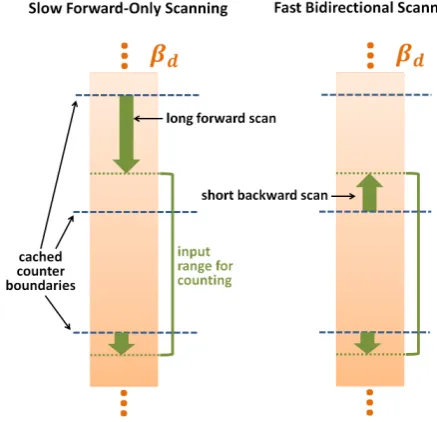
CachingC1 counter values significantly reduces the need for linearly scanning bits ofβd. However, it does not com-pletely eliminate scanning. In order to compute values of C1 for arbitrary inputs, we need to scans bits on average and at most 2sbits with forward scanning (i.e., in order of increasing bit indexes ofβd).

As illustrated in Figure 5, we can further reduce the amount of scanning in half if we extend the algorithm to start from a cached counter boundary and scan backwards until it reaches an edge of the input range. Backward scanning should be performed when the forward scanning length is more than

s/2 (half of the caching stride) and the result should be subtracted from the cached counter value. This optimiza-tion makes it so that the average bits scanned per invocaoptimiza-tion of theC1(and henceC0) functions iss/2 and the maximum iss. The same trick can be used forC−01 andC

−1 1 .

4.2

Counter Alignment

The location of counter boundaries can be slightly shifted to align with the edges of partitions. For example, in

Fig-Figure 5: Performing bidirectional scanning instead of forward-only scanning leads to a 2X speedup of the algorithm.

ure 1, without counter alignment and a stride ofs= 4, we would store counters forC1(β1,0,4) andC1(β1,4,4). If we align the counters, then we can instead store the counters forC1(β1,0,5) andC1(β1,5,3).

Aligning counters helps boost performance. As can be seen in Figures 2 and 3, the algorithm counts the number of ones in the current partition at each level of recursion. Therefore aligning the counters with the partition bound-aries allows the algorithm to count the number of ones bits in a partition by using the cache only and completely avoids linearly scanning the bitstrings in these cases. Moving the cache boundaries comes at a cost of making other C1 oper-ations slightly less efficient, but because less efficient opera-tions occur with lower frequency, counter alignment actually improves the performance of the overall algorithm.

5.

ENHANCEMENTS

5.1

Optimization via Assembly Instructions

−1

1 function. In Section 4, we explain how the amount of scanning can be significantly reduced by caching a small number of counters. However, the scanning cannot be completely eliminated, and the num-ber of bits scanned per invocation ofC0,C1,C−01, orC

−1

1 is

Θ(√NlogN).

We observe that this scanning operation can be performed extremely efficiently with the x86 aesenc, aesenclast, and popcnt assembly instructions. These instructions are avail-able on most modern server, desktop, and laptop processors. On other processors, such as those for mobile phones, the scanning can be done in software without hardware acceler-ation.

andaesenclast instructions which perform one round of an AES encryption as a single instruction. Encrypting a single block takes several rounds (e.g., 10 rounds for 128-bit AES and 14 rounds for 256-bit AES). In our implementation we use 128-bit AES, but this can easily be adjusted (e.g, by adding 4 extra rounds to make it 256-bit).

POPCNT instruction. The popcnt (population count) instruction conveniently allows us to count the number of ones bits in a 64-bit register. Without this instruction, we would need to use less efficient methods such as those in [1].

Example. Suppose that we need to scan β0 to count the number of ones bits inS={β0[0], β0[1], ..., β0[2559]}. Recall that bitsrings are generated by consecutive calls toAESK(·)

with an incrementing index. Specifically,S is the following bitstring:

S=AESK(0)||AESK(1)||AESK(2)||. . .||AESK(19)

The algorithm works as follows: Let c = 0. For i = 0, ...,19, compute AESK(i), count the number of ones bits

in it, and add the count to c. Figure 6 shows assembly code executed for a single value ofi. The indexiis passed in as registerxmm15. The first block of code uses the AES instructionsaesencandaesenclastto computeAESK(i). The

second block of code uses thepopcntinstruction to count the number of bits inAESK(i).

In cases where the bitstring partially covers an AES block, the ones bits in the first and last block of the bitstring can be counted by reading individual bits. The bulk of the AES blocks (in between the first and last block) can still be scanned using the efficient assembly code in Figure 6.

This highly optimized scanning process is used in the im-plementation of the C1 function to scan bitsrings imme-diately before and after cached counter boundaries as de-scribed in Section 4. Similar assembly code can be used to perform the scanning forC0,C−01, andC

−1

1 .

5.2

Cache Compression

The cache for FastPRP can vary from 365 bytes forN = 211 _{to 893KB forN = 2}31_{. Typically, this is a very small} amount of memory usage to get the performance and secu-rity that FastPRP offers. However, in some scenarios, the user may want to store many keys in memory or the amount of memory could be severely limited such as in embedded devices.

Recall that the cache consists of counters for regions of lengths in the bitstrings. Each counter specifies the num-ber of ones in a particular region. Since all of the bits are essentially independent random coin flips, we know that the counter value is a random variable with a binomial distri-bution. Hence the entropy of the counter for the number of ones bits in a region of sizesis

log₂(πes)−1

2 +O

1

s

We can use Huffman codes to compactly store the counter values. This means that, for example, for N = 231 _and

s = 216, we can use about 9 bits per counter on average even though the counters are 16-bit numbers, resulting in about a 57% compression ratio.

5.3

Incremental Caching

; Input AES round keys: xmm0-xmm10 ; Input block ID: xmm15

; Output: rax (# ones in xmm15) ; xmm15 = AesEncrypt(xmm15)

pxor xmm15, xmm0 ; Whitening step (AES Round 0) aesenc xmm15, xmm1 ; AES Round 1

aesenc xmm15, xmm2 ; AES Round 2 aesenc xmm15, xmm3 ; AES Round 3 aesenc xmm15, xmm4 ; AES Round 4 aesenc xmm15, xmm5 ; AES Round 5 aesenc xmm15, xmm6 ; AES Round 6 aesenc xmm15, xmm7 ; AES Round 7 aesenc xmm15, xmm8 ; AES Round 8 aesenc xmm15, xmm9 ; AES Round 9 aesenclast xmm15, xmm10 ; AES Round 10 ; rax = Count ones bits in xmm15 movq r8, xmm15

psrldq xmm15, 8 movq r9, xmm15 popcnt rbx, r8 add rax, rbx popcnt rcx, r9 add rax, rcx

Figure 6: Highly efficient x86-64 assembly instruc-tions for counting the ones bits in a single AES block.

The cache size can always be increased or decreased at run time. For example, if the program is expecting to make lots of PRP invocations in the near future, it can temporarily increase the cache size for improved performance.

It is possible to store the cache in increments where each increment cuts the cache stride in half. For example suppose thatN= 16. In incrementI1, we can cache

I1={C1(βd,0,8),C1(βd,8,8)} and in incrementI2, we can cache

I2={C1(βd,0,4),C1(βd,8,4)}

IncrementI1 is itself a cache with strides= 8. However, we can combineI1andI2to obtain a cache with strides= 4. Note that this is possible because the remaining cache values C1(βd,4,4) andC1(βd,12,4) can be trivially computed from

I1 andI2 without performing any scanning.

Increments can also be stored on disk as separate files and loaded on-demand when higher performance is desired.

6.

EVALUATION

To evaluate our algorithm, we implemented our FastPRP Permute and Unpermute algorithms for arbitrary values of

N. Our implementation uses an adjustable cache size as described in Section 4 and the assembly instruction opti-mizations described in Section 5.1. We chose a cache stride ofs= 2√Nfor our experiments because it offers a balanced tradeoff between the cache size and speed. We ran all of our experiments on the same 4 GHz Intel Core i7 CPU machine.

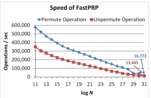
Figure 7: The performance of our construction with cache stride ofs= 2√N.

logN 11 15 21 25 31

Size 365 B 1.9 KB 20 KB 92 KB 893 KB Time (s) <10−6 _<10−6 _{0.001 0.031 2.34}

Table 2: FastPRP cache sizes and cache generation time.

Permute/Unpermute. Figure 7 shows the speed of our algorithm’sPermuteandUnpermuteoperations for domains of sizeN= 211toN= 231. Each data point is an average of 217operations with uniform random inputs. As one would expect, the performance of the algorithm decreases asN in-creases because the recursion depth inin-creases and the cache strides= 2√N increases withN.

TheUnpermuteoperation is slower than thePermute oper-ation because: (1) in our implementoper-ation we did not imple-ment backward scanning forC−01andC

−1

1 functions invoked by Unpermute, and (2) the C−1

0 and C

−1

1 functions do an additional binary search as explained in Section 4.

Cache generation. Generating the cached counters re-quires a scan of bitstrings βd for d = 0,1, . . . ,log2(N/s). This might be concerning because forN= 231, this consists of scanning bitstrings of combined length of 23_{5 bits. Our} results in Table 2 show that the cache generation time is actually quite fast; even forN = 231, it takes about 2.34 seconds on a single core to generate the key. In comparison, it takes about 1.2 seconds to generate a 3072-bit RSA key on the same hardware using OpenSSL. According to NIST [2] a 3072-bit RSA key provides about the same level of security as the 128-bit AES key used by our implementation. It’s important to note that the cache generation only needs to be done once and the cache can then be stored along with the key for future use.

6.2

Comparison to Previous Work

As explained in Section 1.3 and Table 1, the only previ-ous work that achieves as strong security guarantees (with-standingN queries and provable security) as FastPRP is a construction by Granboulan and Pornin [10]. We contacted the authors and they kindly provided us with the implemen-tation that they used in [10]. To achieve a fair comparison, we modified their code to use the same hardware AES in-structions as FastPRP (described in Section 5.1).

Figure 8: Speed comparison between our algorithm and the best previously known algorithm [10] with the same level of security. The “speedup” measured is how many times faster our construction is than the algorithm in [10]. We used cache stride of s= 2√N

for our algorithm.

For domains of sizeN= 211toN= 231, we measured the amount of time it takes FastPRP to perform 217 _Permute andUnpermuteoperations with uniform random inputs. We timed the same operations for [10], but because that algo-rithm is much slower, we used 1000 measurements per data point.

As the results show in Figure 8, our construction is1,000 to 8,000 times fasterthan the best existing construction with the same level of security. Because our algorithm has a higherasymptoticcomplexity than [10], asN keeps increas-ing eventually their construction will become faster. Unfor-tunately, we do not know the exact value of N because de-termining it will require a significant change to their code to handle values with more than 31 bits. However, the graph clearly shows that for N ≤ 231_{, our construction is much} faster in practice.

6.3

Cache Size vs. Speed

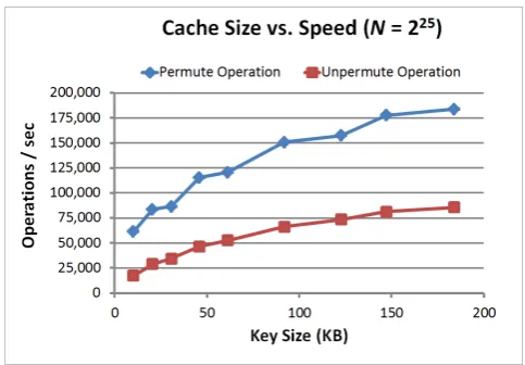
In Figure 9, we demonstrate the tradeoff between cache size and speed of our algorithm. As the cache stride s is decreased for a fixed value domain size (N = 225 in this graph), the cache size increases and so does the speed of the PermuteandUnpermuteoperations. The reason behind this is that a smaller stide between the cached counters reduces the linear scanning work performed by theC0,C1,C−01,C

−1 1 functions.

7.

ASYMPTOTIC ANALYSIS

As mentioned in Section 1, asymptotics is not the most important metric to optimize with small-domain problems. For completeness, in this section, we formally prove that with high probability, the depth of the permute algorithm is bounded byO(logN).

Theorem 2. Letc≥4 log4

3N. With probability at least 1−N·exp(−c/8), the depth of thePermute(orUnpermute) algorithm is bounded byc.

Figure 9: The tradeoff between cache size and speed of FastPRP.

depth for elementiis bounded bycexcept with failure prob-ability exp(−c/8). Next, we apply union bound over the set of all elements inD.

Suppose an elementi∈ D is in some partitionS in the

k-th iteration. This elementi∈ D is calledlucky in thek -th iteration, if -this iteration dividesS into two parts, where both parts contain at mostd3

4|S|eelements. Clearly, element

ican participate in at most log4

3N lucky rounds.

It is not hard to see that any round is a lucky round with probability at least 1

2, for the following reason.

Due to Chernoff bound, in a sequence ofM coin flips, the probability that the number of ones is smaller than M

4 is at most exp(−M/8). Therefore, for rounds where M ≥8, clearly the probabilty of a lucky round is at least 1₂. For

M < 8, it is not hard to verify that the probabilty of a lucky round is at least 1

2 as well.

Due to the Chernoff bound again, in a sequence of c

rounds,

Pr[number of lucky rounds incrounds<1

2c−∆]≤exp(

−2∆2

c )

Let ∆ = 1

2c−log4₃N, we have forc≥4 log4₃N, Pr[number of lucky rounds incrounds<log4

3N] ≤exp(

−2(1

2c−log4₃N) 2

c )≤exp(−c/8)

Now apply union bound for all elements in the universeD, it follows that with probability at least 1−Nexp(−c/8), the depth of thePermute(orUnpermute) algorthm is bounded byc, forc≥log4

3N.

Corollary 2. With probability at least1− 1

Nk, thePermute (orUnpermute) algorithm completes in at most8(k+ 1) lnN

rounds, wherek≥1.

Proof. Letc= 8(k+ 1) lnN in the above theorem, we

get that

Pr[algorithm completes in more than 8(k+ 1) lnN rounds] ≤Nexp(−8(k+ 1) lnN/8)≤ 1

Nk

8.

CONCLUSION AND FUTURE WORK

8.1

Conclusion

We propose a novel construction for a small-domain pseudo-random permutation. As asymptotics is the wrong metric to optimize for small-domain problems, we instead aim for optimal practical performance. Our construction achieves strong security, i.e., can withstand up toN queries from an adversary, and is by far the most efficient construction for 32-bit integers or smaller domains, i.e., (N <232). In par-ticular, our construction is 1,000 to 8,000 times faster than the best known construction achieving a comparable level of security.

8.2

Discussions on Timing Channel and

Fu-ture Work

Just like many other cryptographic algorithms, timing at-tacks can be a serious concern depending on how the algo-rithm is used. An algorithm can withstand timing attacks if every pair of operation that the adversary wishes to dis-tinguish between take the same amount of time to execute. In our algorithm, the bitstring scanning operations domi-nate the execution time of thePermuteandUnpermute algo-rithms. Therefore, in order to defend against timing at-tacks we need to scan the same number of bits regard-less of the inputs. This can easily be done by performing additional dummy scans so the expected number of bits scanned equals the maximum number. If we don’t per-form counter alignment and we use bidirectional scanning, the expected amount of scanning for each invocation of C1 doubles from s/2 to s, introducing a 2X slowdown in the Permute and Unpermute algorithms. With counter align-ment present, the maximum number of bits scanned becomes 2s, but it can be reduced tosby introducing an additional cached counter for the possible input ranges ofC1at depths

d = 0,1, . . . ,log2(N/s). Whens ∈ O( √

N), this increases the key size by a small factor ofO(1/logN).

Timing difference can also be observed due to the varia-tion in the depth of thePermuteandUnpermutealgorithms. Similarly, a padding idea can be applied to hide such vari-ation. In future work, we plan to investigate exactly how much performance penalty will be incurred to perfectly de-fend against timing channel attacks.

Note that in many cases, it may not be necessary to mod-ify the algorithm to defend against timing attacks. The running times of Permuteand Unpermute are many orders of magnitude lower than typical network latency, so often times the fluctuations in execution time will be dominated by fluctuations in network latency.

9.

REFERENCES

[1] Bit Twiddling Hacks.http:

[2] The Case for Elliptic Curve Cryptography.

http://www.nsa.gov/business/programs/elliptic_ curve.shtml.

[3] Tiny encryption algorithm.http://en.wikipedia. org/wiki/Tiny_Encryption_Algorithm.

[4] Xtea.http://en.wikipedia.org/wiki/Tiny_ Encryption_Algorithm.

[5] M. Bellare, T. Ristenpart, P. Rogaway, and T. Stegers. Format-preserving encryption. InSelected Areas in Cryptography, pages 295–312, 2009.

[6] M. Bellare, P. Rogaway, and T. Spies. The ffx mode of operation for format-preserving encryption.

http://csrc.nist.gov/groups/ST/toolkit/BCM/ documents/proposedmodes/ffx/ffx-spec.pdf. [7] J. Black and P. Rogaway. Ciphers with arbitrary finite

domains. InCT-RSA, pages 114–130, 2002. [8] M. Brightwell and H. E. Smith. Using

datatype-preserving encryption to enhance data warehouse security. InNational Information Systems Security Conference (NISSC), 1997.

[9] O. Goldreich and R. Ostrovsky. Software protection and simulation on oblivious rams.J. ACM, 1996. [10] L. Granboulan and T. Pornin. Perfect block ciphers

with small blocks. InFSE, pages 452–465, 2007. [11] M. Luby and C. Rackoff. How to construct

pseudorandom permutations from pseudorandom functions.SIAM J. Comput., 17(2):373–386, Apr. 1988.

[12] U. Maurer and K. Pietrzak. The security of many-round luby-rackoff pseudo-random

permutations. InProceedings of the 22nd international conference on Theory and applications of

cryptographic techniques, EUROCRYPT’03, pages 544–561, Berlin, Heidelberg, 2003. Springer-Verlag. [13] B. Morris, P. Rogaway, and T. Stegers. How to

encipher messages on a small domain. InProceedings of the 29th Annual International Cryptology

Conference on Advances in Cryptology, CRYPTO ’09, pages 286–302. Springer-Verlag, 2009.

[14] J. Patarin. Luby-rackoff: 7 rounds are enough for 2n(1-epsilon)security. InCRYPTO, pages 513–529, 2003.

[15] J. Patarin. Security of random feistel schemes with 5 or more rounds. InCRYPTO, pages 106–122, 2004. [16] V. Pryamikov. Enciphering with arbitrary small finite

domains. InINDOCRYPT, pages 251–265, 2006. [17] R. Schroeppel. Hasty pudding cipher specification.

http://richard.schroeppel.name: 8015/hpc/hpc-spec.